Overview
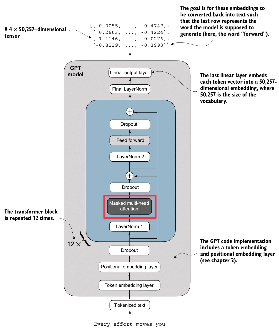
Target GPT & Transformer Architecture
| GPT Architecture | Transformer Architecture |
|---|---|
 |  |
| Source: Build a Large Language Model (From Scratch) - Sebastian Raschka | Source: Build a Large Language Model (From Scratch) - Sebastian Raschka |
Prerequisites
Basic understanding of neural networks is required.
Here’s my article about neuron, activation function, loss function, backpropagation, and gradient descent:
1. Building Blocks
Tokenization
Here’s the Tokenization process (highlighted in red):
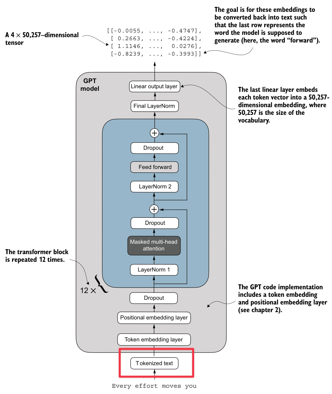
The input to the model is raw text. As shown in the diagram, the system processes a sample sentence like “Every effort moves you” or “Your journey starts with one”.
To process this text computationally, it must be converted into numerical tokens. There are three primary strategies for this conversion:
1. Word-based Tokenization
The simplest approach is to split text by spaces (e.g., ["the", "fox", "chased"]). While intuitive, it has major flaws:
- Out Of Vocabulary (OOV): If the model hasn’t seen the word “internet” during training, it fails.
- No Morphology: It treats words like “boy” and “boys” as completely unrelated concepts, missing their shared root.
- Massive Vocabulary: To cover a language, you need hundreds of thousands of unique tokens.
sample_text = "Tokenization is fun!"
sample_text_2 = "Unhelpful phrasing often hinders understanding."

import re
def demo_word_tokenization(text):
    print("--- Word-based Tokenization ---")
    # Use regex to find words and punctuation separately
    tokens = re.findall(r"\w+|[^\w\s]", text, re.UNICODE)
    print(f"Original text: '{text}'")
    print(f"Tokens: {tokens}")
    print(f"Token count: {len(tokens)}")
    print(f"Unique Tokens: {sorted(set(tokens))}")
    print(f"Unique Token count: {len(set(tokens))}")
    print("-" * 30)

demo_word_tokenization(sample_text)
demo_word_tokenization(sample_text_2)
Output:
--- Word-based Tokenization ---
Original text: 'Tokenization is fun!'
Tokens: ['Tokenization', 'is', 'fun', '!']
Token count: 4
Unique Tokens: ['!', 'Tokenization', 'fun', 'is']
Unique Token count: 4
------------------------------

--- Word-based Tokenization ---
Original text: 'Unhelpful phrasing often hinders understanding.'
Tokens: ['Unhelpful', 'phrasing', 'often', 'hinders', 'understanding', '.']
Token count: 6
Unique Tokens: ['.', 'Unhelpful', 'hinders', 'often', 'phrasing', 'understanding']
Unique Token count: 6
------------------------------
2. Character-based Tokenization
We could go smaller and split by character (e.g., ['t', 'h', 'e']).
- Pros: Small vocabulary (just ~256 characters) and no OOV issues (you can spell anything).
- Cons: Loss of Meaning (an ‘a’ has no semantic value) and Inefficiency. A simple word like “dinosaur” becomes 8 tokens, making sequences processing computationally expensive.
sample_text = "Tokenization is fun!"
sample_text_2 = "Unhelpful phrasing often hinders understanding."

def demo_char_tokenization(text):
    print("\n--- Character-based Tokenization ---")
    tokens = list(text)
    print(f"Original text: '{text}'")
    print(f"Tokens: {tokens}")
    print(f"Token count: {len(tokens)}")
    print(f"Unique Tokens: {sorted(set(tokens))}")
    print(f"Unique Token count: {len(set(tokens))}")
    print("-" * 30)

demo_char_tokenization(sample_text)
demo_char_tokenization(sample_text_2)
Output:
--- Character-based Tokenization ---
Original text: 'Tokenization is fun!'
Tokens: ['T', 'o', 'k', 'e', 'n', 'i', 'z', 'a', 't', 'i', 'o', 'n', ' ', 'i', 's', ' ', 'f', 'u', 'n', '!']
Token count: 20
Unique Tokens: [' ', '!', 'T', 'a', 'e', 'f', 'i', 'k', 'n', 'o', 's', 't', 'u', 'z']
Unique Token count: 14
------------------------------

--- Character-based Tokenization ---
Original text: 'Unhelpful phrasing often hinders understanding.'
Tokens: ['U', 'n', 'h', 'e', 'l', 'p', 'f', 'u', 'l', ' ', 'p', 'h', 'r', 'a', 's', 'i', 'n', 'g', ' ', 'o', 'f', 't', 'e', 'n', ' ', 'h', 'i', 'n', 'd', 'e', 'r', 's', ' ', 'u', 'n', 'd', 'e', 'r', 's', 't', 'a', 'n', 'd', 'i', 'n', 'g', '.']
Token count: 47
Unique Tokens: [' ', '.', 'U', 'a', 'd', 'e', 'f', 'g', 'h', 'i', 'l', 'n', 'o', 'p', 'r', 's', 't', 'u']
Unique Token count: 18
------------------------------
3. Subword-based Tokenization (BPE)
Modern LLMs use a hybrid approach called Byte Pair Encoding (BPE). It strikes a balance by following two rules:
- Frequent words are kept intact as single tokens (like “Your” ->
1639). - Rare words are split into meaningful chunks (morphology). For example, “tokenization” might become
["token", "ization"].
This “best of both worlds” strategy allows GPT-2 to maintain a manageable vocabulary of 50,257 while handling any English text efficiently.
For example, in our diagram:
- The common word “Your” maps directly to ID
1639. - The space-prefixed word ” journey” maps to
10950.
This results in a tensor of shape (Batch, Sequence_Length), specifically (1, 5) in this example.
sample_text = "Tokenization is fun!"
sample_text_2 = "Unhelpful phrasing often hinders understanding."

import tiktoken
def demo_subword_tokenization(text):
    print("\n--- Subword-based Tokenization (using tiktoken) ---")
    try:
        enc = tiktoken.get_encoding("cl100k_base")
        tokens = enc.encode(text)
        token_bytes = [enc.decode_single_token_bytes(token) for token in tokens]
        print(f"Original text: '{text}'")
        print(f"Tokens (IDs): {tokens}")
        print(f"Tokens (Bytes): {token_bytes}")
        print(f"Token count: {len(tokens)}")
        print(f"Unique Tokens (IDs): {sorted(set(tokens))}")
        # Sorting bytes might need care, but sorted() works on list of bytes
        print(f"Unique Tokens (Bytes): {sorted(set(token_bytes))}")
        print(f"Unique Token count: {len(set(tokens))}")
    except ImportError:
        print("tiktoken not installed. Please install it to see subword tokenization.")
    print("-" * 30)

demo_subword_tokenization(sample_text)
demo_subword_tokenization(sample_text_2)
Output:
--- Subword-based Tokenization (using tiktoken) ---
Original text: 'Tokenization is fun!'
Tokens (IDs): [3404, 2065, 374, 2523, 0]
Tokens (Bytes): [b'Token', b'ization', b' is', b' fun', b'!']
Token count: 5
Unique Tokens (IDs): [0, 374, 2065, 2523, 3404]
Unique Tokens (Bytes): [b' fun', b' is', b'!', b'Token', b'ization']
Unique Token count: 5
------------------------------

--- Subword-based Tokenization (using tiktoken) ---
Original text: 'Unhelpful phrasing often hinders understanding.'
Tokens (IDs): [1844, 8823, 1285, 1343, 97578, 3629, 305, 32551, 8830, 13]
Tokens (Bytes): [b'Un', b'help', b'ful', b' ph', b'rasing', b' often', b' h', b'inders', b' understanding', b'.']
Token count: 10
Unique Tokens (IDs): [13, 305, 1285, 1343, 1844, 3629, 8823, 8830, 32551, 97578]
Unique Tokens (Bytes): [b' h', b' often', b' ph', b' understanding', b'.', b'Un', b'ful', b'help', b'inders', b'rasing']
Unique Token count: 10
------------------------------
Embeddings
Here’s the Embeddings process (highlighted in red):
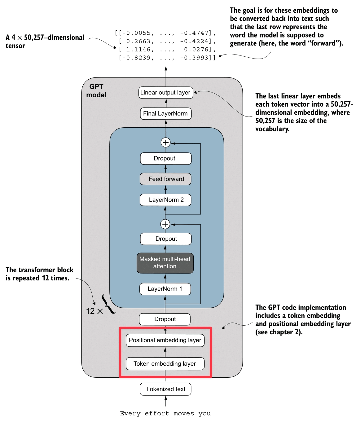
The output of our BPE Tokenizer and DataLoader is a batch of integer arrays—specifically, (Batch, Context_Size) tensors of Token IDs (e.g., [1639, 10950, ...]). However, to a neural network, the integer 1639 (“Your”) is arbitrarily larger than 287 (“the”). There is no inherent mathematical relationship between these numbers.
To address this, we transform these IDs into dense vectors using Embeddings. This process maps each token ID to a high-dimensional vector space, where similar tokens are closer to each other mathematically.
For example, let’s consider the following word analogy:
If we treat words as vectors, we can perform arithmetic on them. By subtracting the ‘male’ concept from ‘King’ and adding the ‘female’ concept, we should mathematically arrive at ‘Queen’.
Let’s use the Word2Vec model from Gensim to compute the answer.
import gensim.downloader as api

# Load the Word2Vec model
wv = api.load('word2vec-google-news-300')

# The most_similar function finds the top N closest vectors to the result of (positive - negative)
result = wv.most_similar(positive=['king', 'woman'], negative=['man'], topn=1)
print(f"King - Man + Woman = {result[0][0]} (Similarity: {result[0][1]:.2f})")
Output:
King - Man + Woman =
queen (Similarity: 0.71)
The closest word to the result of (king - man + woman) is queen.
The output confirms that the model successfully captured the gender relationship. Beyond arithmetic, we can also compute the cosine similarity between any two words to measure how semantically close they are. For example:
sim_paper_water = wv.similarity('paper', 'water')
sim_man_woman = wv.similarity('man', 'woman')

print(f"Similarity between 'paper' and 'water': {sim_paper_water:.2f}")
print(f"Similarity between 'man' and 'woman':   {sim_man_woman:.2f}")
Output:
Similarity between 'paper' and 'water': 0.11
Similarity between 'man' and 'woman':   0.77
If we just use raw token IDs, 10 is very close to 11. But in language, “apple” (10) might be very different from “apply” (11). We need a bridge that converts these discrete IDs into a continuous space where “cat” and “kitten” are mathematically close.
1. Token Embedding
The Token Embedding layer is a trainable lookup table. It maps each integer token ID to a dense vector of floating-point numbers.
- Input: Token IDs (Integers)
- Output: Dense Vectors (Floats) which encode semantic meaning.
If visualization helps, think of it as a massive Excel sheet where:
- Rows = Vocabulary Size (50,257 for GPT-2)
- Columns = Embedding Dimension (768 for GPT-2 Small)
Each row represents the “meaning” of a token. Initially, these are random noise. As the model trains, it updates these numbers so that synonyms drift closer together in this 768-dimensional space.
# Create the Token Embedding Layer
# vocab_size = 50257
# emb_dim = 768
token_embedding_layer = nn.Embedding(vocab_size, emb_dim)
2. Positional Embedding
While Token Embeddings capture what a word is, they fail to capture where it is. “The cat sat on the mat” vs “The mat sat on the cat”. To the model, these are just bags of identical vectors. The meaning is lost because the order is ignored.
To fix this, we inject Positional Information. We create another lookup table, but this time for positions (0, 1, 2, … 1023).
- Input: Position IDs (0, 1, 2…)
- Output: Positional Vectors
These vectors are simply added to the token embeddings.
Now, the vector for “cat” at position 2 is slightly different from the vector for “cat” at position 6. This subtle difference allows the Transformer to distinguish order.
# Create the Positional Embedding Layer
# context_length = 1024 (Max sequence length)
# emb_dim = 768
pos_embedding_layer = nn.Embedding(context_length, emb_dim)

# Input construction
pos_embeddings = pos_embedding_layer(torch.arange(seq_len)) # [0, 1, 2...]
final_embeddings = token_embeddings + pos_embeddings
Attention Mechanism
Here’s the Attention Mechanism process (highlighted in red):
The Attention Mechanism is the core engine of the Transformer. It allows the model to “focus” on relevant parts of the input sequence when processing a specific token.
In this section, we will build the attention mechanism from scratch in three steps:
- Simplified Self-Attention: Understanding the core concept without trainable weights.
- Self-Attention with Trainable Weights: Adding
Query,Key, andValuematrices to let the model learn relationships. - Masked Self-Attention: Ensuring the model can’t see the future (crucial for GPT).
- Multi-Head Attention: Running multiple attention heads in parallel to capture different types of relationships.
Dot Product and Similarity
Before diving into attention, we need to understand the Dot Product. It is the fundamental operation used to measure similarity between two vectors.
The dot product of two vectors and is defined as:
- Aligned (): Dot product is large positive. (High Similarity)
- Perpendicular (): Dot product is zero. (No Similarity)
- Opposite (): Dot product is large negative.
In the context of the Attention Mechanism, a high dot product between two token vectors means they are related, and the model should pay more “attention” to that relationship.
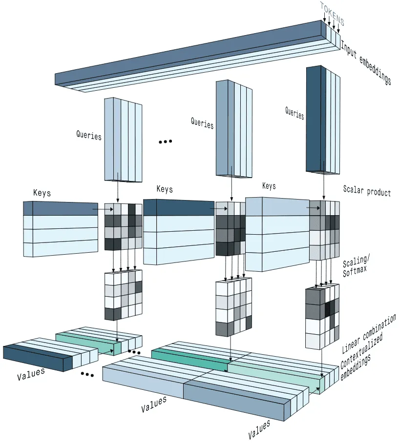
Simplified Attention Mechanism (Without QKV)
In this simplified version, we don’t use any trainable weights. We just use the raw embedding vectors to calculate similarity.
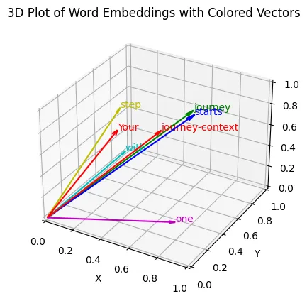
Let’s take the sentence: “Your journey starts with one step”. We want to compute a new vector for “journey” that captures its relationship with other words in the sentence.
Step 1: Computing Attention Scores
We calculate the similarity between “journey” and every other word in the sentence using the dot product.
For this example, let’s assign simple 3D vectors to our words:
- “Your” ():
[0.43, 0.15, 0.89] - “journey” ():
[0.55, 0.87, 0.66] - “starts” ():
[0.57, 0.85, 0.64] - “with” ():
[0.22, 0.58, 0.33] - “one” ():
[0.77, 0.25, 0.10] - “step” ():
[0.05, 0.80, 0.55]
Then, let’s compute the dot product for “journey” against the others to see how similar they are:
-
“journey” “starts”: (High Similarity)
-
“journey” “one”: (Low Similarity)
These raw values are the Attention Scores.
Step 2: Computing Attention Weights
Next, we normalize these scores using the Softmax function to get Attention Weights. They represent the percentage or fraction of attention the model should pay to each input token for a given query (in this case “journey”).
Attention Weights to “journey” (rounded):
- “Your”: 0.14 (14%)
- “journey”: 0.24 (24%)
- “starts”: 0.23 (23%)
- “with”: 0.12 (12%)
- “one”: 0.11 (11%)
- “step”: 0.16 (16%)
- Sum: 1.0 (100%)
Step 3: Computing Context Vectors
Finally, we create the Context Vector for “journey”. It is a weighted sum of all input vectors.
The resulting vector captures the meaning of “journey” enriched with the context of this sentence than the original vector .
Implementation
import torch
import torch.nn as nn

class SelfAttentionWithoutQKV(nn.Module):
    def __init__(self):
        super().__init__()

    def forward(self, x):
        # x dimensions: [num_tokens, d_in]
        # Step 1: Compute raw attention scores
        attn_scores = x @ x.T

        # Step 2: Normalize with Softmax
        attn_weights = torch.softmax(attn_scores, dim=-1)

        # Step 3: Compute Context Vectors
        context_vec = attn_weights @ x
        return context_vec

# Define the input vectors (embeddings) for the sentence: "Your journey starts with one step"
# Values taken from the blog post example
inputs = torch.tensor([
    [0.43, 0.15, 0.89], # Your    (x1)
    [0.55, 0.87, 0.66], # journey (x2)
    [0.57, 0.85, 0.64], # starts  (x3)
    [0.22, 0.58, 0.33], # with    (x4)
    [0.77, 0.25, 0.10], # one     (x5)
    [0.05, 0.80, 0.55]  # step    (x6)
])

# Initialize the module
sa_simple = SelfAttentionWithoutQKV()

# Compute context vectors
context_vectors = sa_simple(inputs)

print("SelfAttentionWithoutQKV Output (Context Vectors):")
print(context_vectors)

print("\nSpecific Context Vector for 'journey':")
print(context_vectors[1])
Result:
SelfAttentionWithoutQKV Output (Context Vectors):
tensor([[0.4421, 0.5931, 0.5790],
        [0.4419, 0.6515, 0.5683],
        [0.4431, 0.6496, 0.5671],
        [0.4304, 0.6298, 0.5510],
        [0.4671, 0.5910, 0.5266],
        [0.4177, 0.6503, 0.5645]])

Specific Context Vector for 'journey':
tensor([0.4419, 0.6515, 0.5683])
Self-Attention with Trainable Weights (QKV)
In real LLMs, we don’t simply use the raw input embeddings. We want the model to learn how to attend. To do this, we introduce three trainable weight matrices: (Query), (Key), and (Value).
Step 1: Projection (Trainable Weights)
We project the input vector into three distinct vectors:
- Query (): What am I looking for?
- Key (): What do I contain? (Used for matching)
- Value (): What information do I pass along?
For this example, we initialize our three weight matrices with random values (using seed 123):
Let’s look at the projected vectors for “journey” and “starts” from our example:
Step 2: Computing Attention Scores
We calculate the similarity between the Query of the current token and the Keys of all other tokens.
For instance, the score between “journey” (Query) and “starts” (Key) is calculated as:
Step 3: Computing Attention Weights
We normalize the scores using Softmax, but with a twist: we divide by (dimension of keys).
For our specific score of 0.26, the scaling step looks like this:
(This is done for all words in the sequence, and then Softmax is applied to get the final weights).
Here are the Scaled Scores (Logits) for “journey” against all words:
- “Your”: 0.12
- “journey”: 0.18
- “starts”: 0.18
- “with”: 0.10
- “one”: 0.10
- “step”: 0.13
After applying Softmax, we get the final Attention Weights:
- “Your”: 0.16
- “journey”: 0.17
- “starts”: 0.17
- “with”: 0.16
- “one”: 0.16
- “step”: 0.17
- Sum: ~1.0
The values are close to each other because our random weights produced similar dot products. In a trained model, these would be much more distinct!
Step 4: Computing Context Vectors
We use the weights to aggregate the Values (not the raw inputs).
The Context Vector for “journey” is computed as:
Implementation
class SelfAttentionQKV(nn.Module):
    def __init__(self, d_in, d_out):
        super().__init__()
        # Use nn.Linear instead of manual nn.Parameter
        self.W_query = nn.Linear(d_in, d_out, bias=False)
        self.W_key   = nn.Linear(d_in, d_out, bias=False)
        self.W_value = nn.Linear(d_in, d_out, bias=False)

    def forward(self, x):
        # Step 1: Project inputs to Q, K, V
        keys = self.W_key(x)
        queries = self.W_query(x)
        values = self.W_value(x)

        # Step 2: Calculate Scores (Queries @ Keys_Transpose)
        # We use transpose(-2, -1) to swap the last two dimensions
        attn_scores = queries @ keys.transpose(-2, -1)

        # Step 3: Scale and Normalize
        d_k = keys.shape[-1]
        attn_weights = torch.softmax(
            attn_scores / d_k**0.5, dim=-1
        )

        # Step 4: Weighted Sum of Values
        context_vec = attn_weights @ values
        return context_vec

d_in = 3
d_out = 2
torch.manual_seed(123)
sa = SelfAttentionQKV(d_in, d_out)
print("SelfAttentionQKV Output:\n", sa(inputs))
Result:
SelfAttentionQKV Output:
tensor([[-0.5337, -0.1051],
        [-0.5323, -0.1080],
        [-0.5323, -0.1079],
        [-0.5297, -0.1076],
        [-0.5311, -0.1066],
        [-0.5299, -0.1081]], grad_fn=<MmBackward0>)
WHY DIVIDE BY SQRT (DIMENSION)?
We scale the dot products by before Softmax.
Reason 1: For stability in learning
If dot products are too large, the Softmax function becomes “peaky” (one value is 1, others 0). This causes gradients to vanish, killing the learning process.
import torch

# Define the tensor
tensor = torch.tensor([0.1, -0.2, 0.3, -0.2, 0.5])

# Apply softmax without scaling
softmax_result = torch.softmax(tensor, dim=-1)
print("Softmax without scaling:", softmax_result)

# Multiply the tensor by 8 and then apply softmax
scaled_tensor = tensor * 8
softmax_scaled_result = torch.softmax(scaled_tensor, dim=-1)
print("Softmax after scaling (tensor * 8):", softmax_scaled_result)
Result:
Softmax without scaling: tensor([0.1925, 0.1426, 0.2351, 0.1426, 0.2872])
Softmax after scaling (tensor * 8): tensor([0.0326, 0.0030, 0.1615, 0.0030, 0.8000])
Reason 2: To make the variance of the dot product stable
Multiplying two random vectors increases variance. As dimension grows, the variance of the dot product grows. Dividing by keeps the variance close to 1, regardless of vector size.
import numpy as np

# Function to compute variance before and after scaling
def compute_variance(dim, num_trials=1000):
    dot_products = []
    scaled_dot_products = []

    # Generate multiple random vectors and compute dot products
    for _ in range(num_trials):
        q = np.random.randn(dim)
        k = np.random.randn(dim)

        # Compute dot product
        dot_product = np.dot(q, k)
        dot_products.append(dot_product)

        # Scale the dot product by sqrt(dim)
        scaled_dot_product = dot_product / np.sqrt(dim)
        scaled_dot_products.append(scaled_dot_product)

    # Calculate variance of the dot products
    variance_before_scaling = np.var(dot_products)
    variance_after_scaling = np.var(scaled_dot_products)

    return variance_before_scaling, variance_after_scaling

# For dimension 5
variance_before_5, variance_after_5 = compute_variance(5)
print(f"Variance before scaling (dim=5): {variance_before_5}")
print(f"Variance after scaling (dim=5): {variance_after_5}")

# For dimension 100
variance_before_100, variance_after_100 = compute_variance(100)
print(f"Variance before scaling (dim=100): {variance_before_100}")
print(f"Variance after scaling (dim=100): {variance_after_100}")
Result:
Variance before scaling (dim=5): 5.392240066108794
Variance after scaling (dim=5): 1.0784480132217587
Variance before scaling (dim=100): 100.67940063891818
Variance after scaling (dim=100): 1.0067940063891818
Causal Self-Attention
In the previous “Self-Attention” mechanism, when we processed the word “journey”, we allowed it to look at “starts”, “with”, “one”, and all future words.
Step 1: “Your” -> “journey” (OK) Step 2: “journey” -> “starts” (Wait, this is cheating!)
If we are training a model to predict the next word, allowing it to see the future words (like “starts”) is cheating. It would just copy the next word instead of learning the language structure.
To fix this, we need to mask the future. When the model is at “journey”, it should only be allowed to see “Your” and “journey”. It should represent:
- “Your”: Can see “Your”
- “journey”: Can see “Your”, “journey”
- “starts”: Can see “Your”, “journey”, “starts”
This creates a triangular pattern of visibility.
Triangular Matrix
How do we strictly enforce this in mathematics? We use a Mask (Upper Triangular Matrix) filled with negative infinity ().
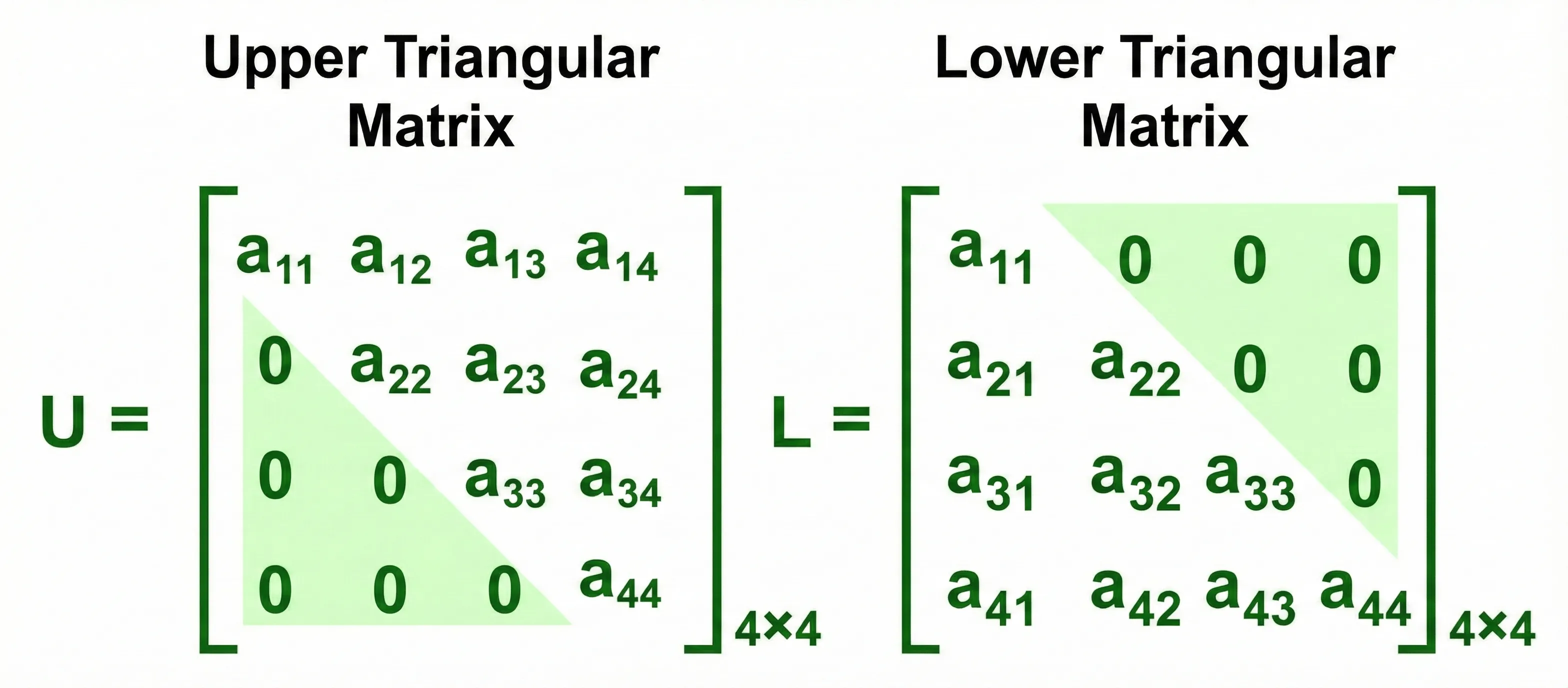
Triangular Matrices
We calculate the Attention Scores as usual, but before applying Softmax, we “add” this mask to the scores.
For example, looking at the scores for the first 3 words (“Your”, “journey”, “starts”):
Then, when we apply Softmax:
This ensures the probability (attention weight) for any future word becomes exactly 0.
Notice how each row sums to 1, and the upper triangle is strictly zero. These are the Attention Weights. The final Context Vector is computed by multiplying these weights with the Value () vectors.
Implementation
import torch
import torch.nn as nn

class CausalAttention(nn.Module):
    def __init__(self, d_in, d_out, context_length, dropout, qkv_bias=False):
        super().__init__()
        self.d_out = d_out
        self.W_query = nn.Linear(d_in, d_out, bias=qkv_bias)
        self.W_key   = nn.Linear(d_in, d_out, bias=qkv_bias)
        self.W_value = nn.Linear(d_in, d_out, bias=qkv_bias)
        self.dropout = nn.Dropout(dropout)
        # Create a causal mask (upper triangular matrix)
        # We register it as a buffer so it's part of the state_dict but not a trained parameter
        self.register_buffer('mask', torch.triu(torch.ones(context_length, context_length), diagonal=1))

    def forward(self, x):
        # Handle batch dimension
        b, num_tokens, d_in = x.shape

        keys = self.W_key(x)
        queries = self.W_query(x)
        values = self.W_value(x)

        # Transpose keys for dot product: (b, num_tokens, d_out) -> (b, d_out, num_tokens)
        # We transpose the last two dimensions to facilitate queries @ keys^T
        attn_scores = queries @ keys.transpose(1, 2)

        # Apply Mask
        # We use masked_fill to set positions where mask is 1 (upper triangle) to -inf
        # We slice the mask to match the current sequence length (num_tokens)
        attn_scores.masked_fill_(
            self.mask.bool()[:num_tokens, :num_tokens], -torch.inf
        )

        attn_weights = torch.softmax(
            attn_scores / keys.shape[-1]**0.5, dim=-1
        )
        attn_weights = self.dropout(attn_weights)

        context_vec = attn_weights @ values
        return context_vec, attn_weights

torch.manual_seed(123)

# Define the input vectors (same as before)
inputs = torch.tensor([
    [0.43, 0.15, 0.89], # Your    (x1)
    [0.55, 0.87, 0.66], # journey (x2)
    [0.57, 0.85, 0.64], # starts  (x3)
    [0.22, 0.58, 0.33], # with    (x4)
    [0.77, 0.25, 0.10], # one     (x5)
    [0.05, 0.80, 0.55]  # step    (x6)
])

# Create a batch input (2 batches of the same input)
batch = torch.stack((inputs, inputs), dim=0)

d_in = 3
d_out = 2
context_length = batch.shape[1]
causal_attn = CausalAttention(d_in, d_out, context_length, dropout=0.0)

context_vecs, attn_weights = causal_attn(batch)

print("Causal Attention Output Shape:", context_vecs.shape)
print("\nAttention Weights for the first batch, 'journey' token (row 1):")
# We expect 'journey' (index 1) to only attend to 'Your' (0) and 'journey' (1)
print(attn_weights[0, 1].tolist())

print("\nFull Attention Weights Matrix (First Batch):")
print(attn_weights[0])
Result:
Causal Attention Output Shape: torch.Size([2, 6, 2])

Attention Weights for the first batch, 'journey' token (row 1):
[0.48326990008354187, 0.5167301297187805, 0.0, 0.0, 0.0, 0.0]

Full Attention Weights Matrix (First Batch):
tensor([[1.0000, 0.0000, 0.0000, 0.0000, 0.0000, 0.0000],
        [0.4833, 0.5167, 0.0000, 0.0000, 0.0000, 0.0000],
        [0.3190, 0.3408, 0.3402, 0.0000, 0.0000, 0.0000],
        [0.2445, 0.2545, 0.2542, 0.2468, 0.0000, 0.0000],
        [0.1994, 0.2060, 0.2058, 0.1935, 0.1953, 0.0000],
        [0.1624, 0.1709, 0.1706, 0.1654, 0.1625, 0.1682]],
       grad_fn=<SelectBackward0>)
Multi-Head Self-Attention
Multi-Head Attention is essentially running multiple instances of Causal Self-Attention in parallel.
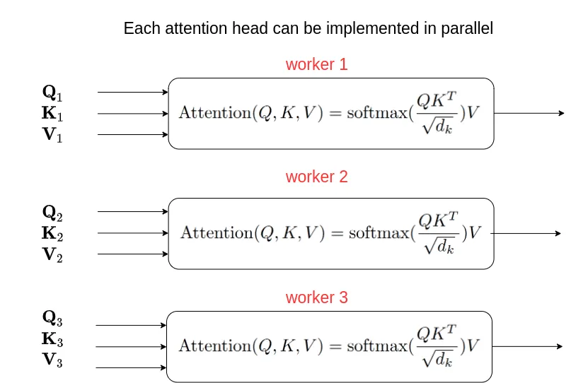
Multi-Head Self-Attention Block Diagram
Source: Why multi-head self attention works: math, intuitions and 10+1 hidden insights | AI Summer
Multi-Head Attention Diagram
Source: Why multi-head self attention works: math, intuitions and 10+1 hidden insights | AI Summer
Multiple Experts
Why do we need multiple heads? Think about understanding a complex sentence. You need to focus on multiple things at once:
- Grammar: How “Journey” connects to “Starts” (Subject-Verb).
- Context: How “Your” describes “Journey” (Adjective-Noun).
If we only had one “Head” (one set of Q, K, V), the model would have to mix all these different relationships into a single average. Creating multiple heads allows each head to become an “expert” in a specific type of relationship.
Instead of having just one set of Query, Key, and Value matrices, we give the model multiple sets. This allows Head 1 to focus on grammar while Head 2 focuses on context, without interfering with each other.
Weight Split Technique
- The Slow Way: If we had 2 heads, we would need 2 separate sets of matrices. That means matrix multiplications.
- The Fast Way (Weight Splits): We use one large matrix for and then splitting the result. This means only 3 matrix multiplications, no matter how many heads we have!
Step-by-Step Trace with Values ():
Let’s follow the second token “journey” () and see how it attends to “Your” () and itself.
- Input: (Shape:
1x1x3)
Step 1. Linear Projection
We project input size 3 to output size 2.
- Result: (Shape:
1x1x2)
Step 2. Tensor Unrolling (Split Heads)
We split the 2-dimensional vector into two 1-dimensional heads.
- Head 1 gets index 0:
- Head 2 gets index 1:
- Shape:
(1, 1, 2, 1)(Batch, Tokens, Heads, Head_Dim)
Step 3. Transpose
We swap dimensions so we can group by head.
- Head 1’s View (Keys):
- Head 2’s View (Keys):
Now Head 1 can compare “journey” against “Your” and “journey” in parallel.
Step 4. Parallel Attention (Focus on Head 1)
- Query:
- Score vs “Your”:
- Score vs “journey”:
- Softmax Weights:
- “Your”
- “journey”
Step 5. Weighted Sum (The “Value” Step)
- Head 1 Value for “Your”:
- Head 1 Value for “journey”:
- Calculation:
(Head 2 does its own independent calculation to get )
Step 6. Concatenation
We glue the head results back together.
- Combined Vector: (Shape:
1x1x2)
Now, we have a single enriched vector that contains insights from multiple heads that are specialized in different aspects of the input.
Implementation
class MultiHeadAttention(nn.Module):
    def __init__(self, d_in, d_out, context_length, dropout, num_heads, qkv_bias=False):
        super().__init__()
        assert (d_out % num_heads == 0), \
            "d_out must be divisible by num_heads"

        self.d_out = d_out
        self.num_heads = num_heads
        self.head_dim = d_out // num_heads # Reduce the projection dim

        self.W_query = nn.Linear(d_in, d_out, bias=qkv_bias)
        self.W_key = nn.Linear(d_in, d_out, bias=qkv_bias)
        self.W_value = nn.Linear(d_in, d_out, bias=qkv_bias)
        self.out_proj = nn.Linear(d_out, d_out)  # Linear layer to combine head outputs
        self.dropout = nn.Dropout(dropout)
        self.register_buffer(
            "mask",
            torch.triu(torch.ones(context_length, context_length),
                       diagonal=1)
        )

    def forward(self, x):
        b, num_tokens, d_in = x.shape

        keys = self.W_key(x) # Shape: (b, num_tokens, d_out)
        queries = self.W_query(x)
        values = self.W_value(x)

        # We implicitly split the matrix by adding a `num_heads` dimension
        # Unroll last dim: (b, num_tokens, d_out) -> (b, num_tokens, num_heads, head_dim)
        keys = keys.view(b, num_tokens, self.num_heads, self.head_dim)
        values = values.view(b, num_tokens, self.num_heads, self.head_dim)
        queries = queries.view(b, num_tokens, self.num_heads, self.head_dim)

        # Transpose: (b, num_tokens, num_heads, head_dim) -> (b, num_heads, num_tokens, head_dim)
        # This puts heads in a dimension where we can parallelize
        keys = keys.transpose(1, 2)
        queries = queries.transpose(1, 2)
        values = values.transpose(1, 2)

        # Compute scaled dot-product attention
        # Corresponds to queries @ keys.T for each head
        attn_scores = queries @ keys.transpose(2, 3)

        # Apply Causal Mask
        mask_bool = self.mask.bool()[:num_tokens, :num_tokens]
        attn_scores.masked_fill_(mask_bool, -torch.inf)

        attn_weights = torch.softmax(attn_scores / keys.shape[-1]**0.5, dim=-1)
        attn_weights = self.dropout(attn_weights)

        # Context vector computation
        # shape: (b, num_heads, num_tokens, head_dim)
        context_vec = (attn_weights @ values).transpose(1, 2)

        # Combine heads
        # contiguous() is needed before view() if memory layout was changed by transpose
        context_vec = context_vec.contiguous().view(b, num_tokens, self.d_out)

        print(f"Context Vector for 'journey' (before final proj): {context_vec[0, 1].detach().numpy()}")

        context_vec = self.out_proj(context_vec)

        return context_vec

mha = MultiHeadAttention(d_in=3, d_out=2, context_length=6, dropout=0.0, num_heads=2)
output = mha(batch)
print("Multi-Head Attention Output:\n", output)
print("Output Shape:", output.shape)
Result:
Context Vector for 'journey' (before final proj): [-0.5872  0.0124]
Multi-Head Attention Output:
tensor([[[0.3190, 0.4858],
         [0.2943, 0.3897],
         [0.2856, 0.3593],
         [0.2693, 0.3873],
         [0.2639, 0.3928],
         [0.2575, 0.4028]],

        [[0.3190, 0.4858],
         [0.2943, 0.3897],
         [0.2856, 0.3593],
         [0.2693, 0.3873],
         [0.2639, 0.3928],
         [0.2575, 0.4028]]], grad_fn=<ViewBackward0>)
Output Shape: torch.Size([2, 6, 2])
Dropout
Here’s the Dropout process (highlighted in red):
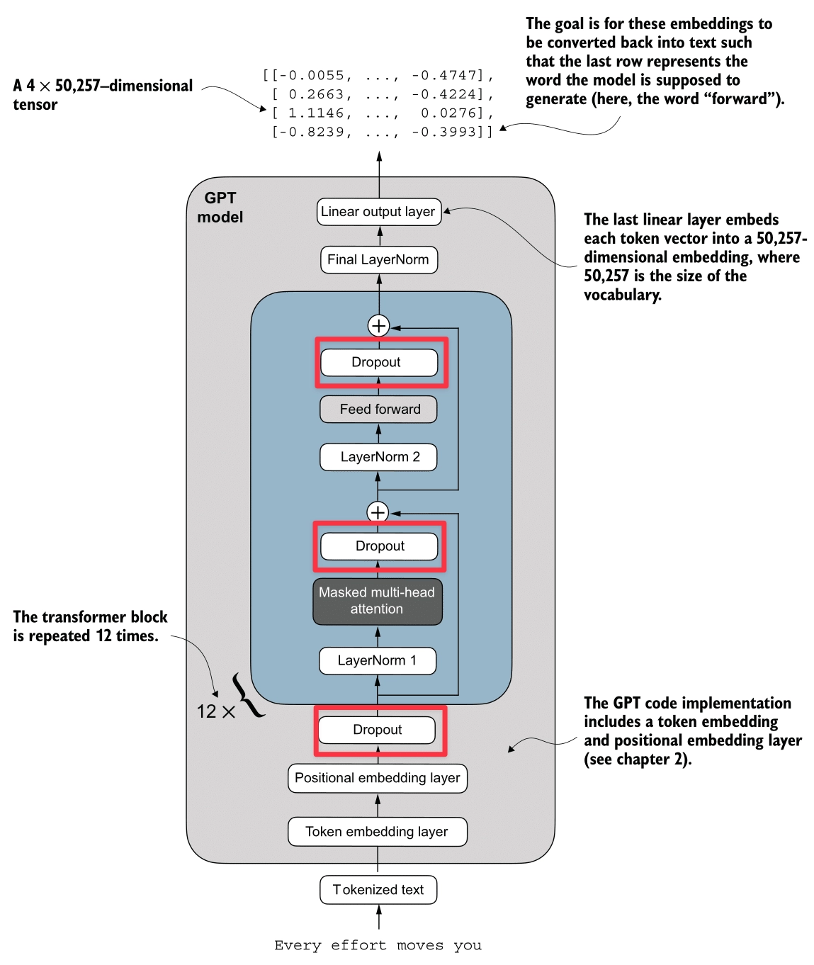
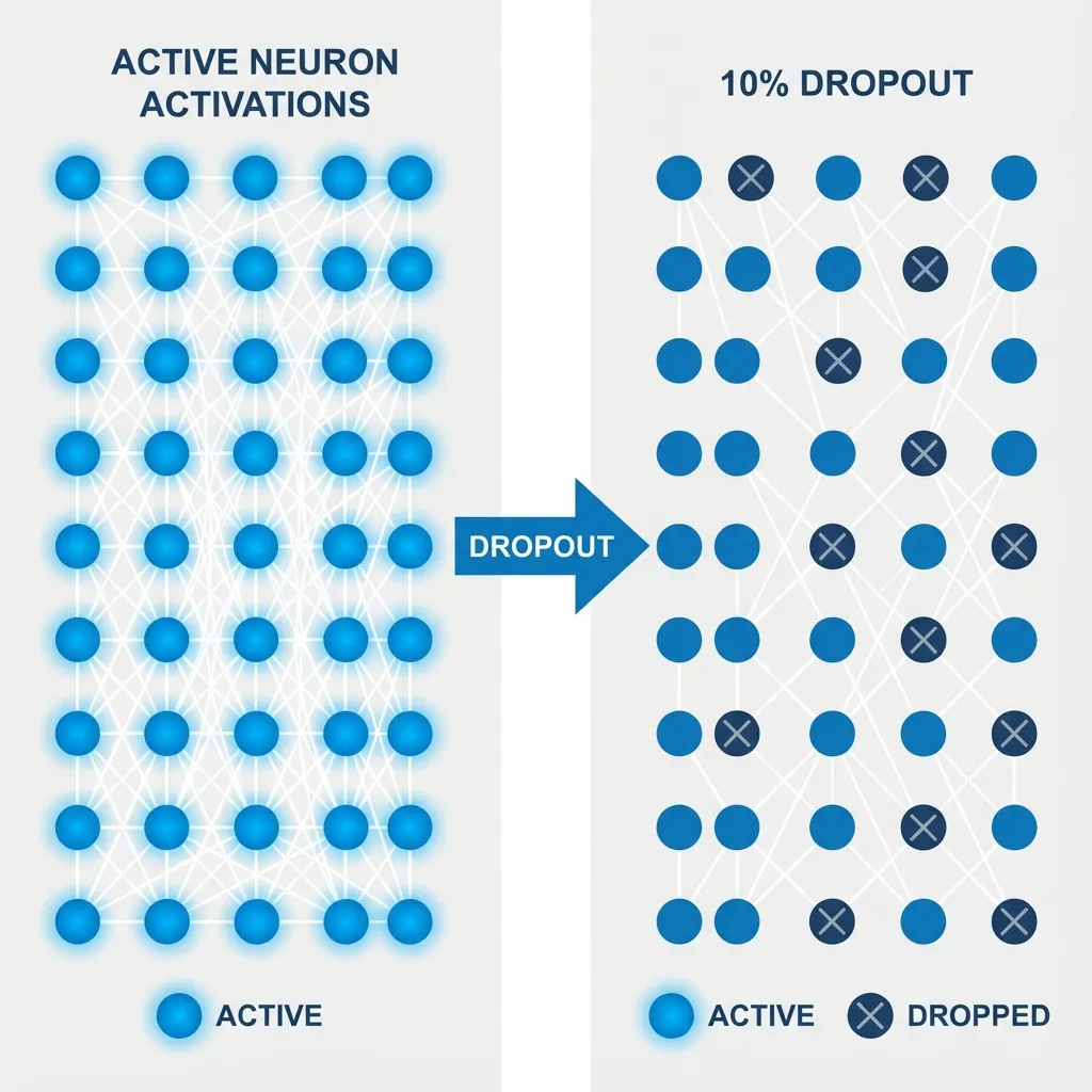
Dropout is a regularization technique used to prevent overfitting.
It works by randomly “switching off” (zeroing out) some of the attention weights during training.
- Mechanism: After calculating the Softmax scores (probabilities), we apply a dropout mask. If a weight is dropped, it becomes 0.
- Effect: This forces the model to not rely too heavily on any single token for context, encouraging it to learn more robust distributed representations.
- Scaling: To keep the expected magnitude of the values constant, the remaining active weights are scaled up (divided by ).
Implementation
input_embeddings = token_embeddings + pos_embeddings

# Dropout layer (e.g., 10% dropout)
dropout = nn.Dropout(0.1)

# Apply dropout
output = dropout(input_embeddings)
Layer Normalization
Here’s the Layer Normalization process (highlighted in red):
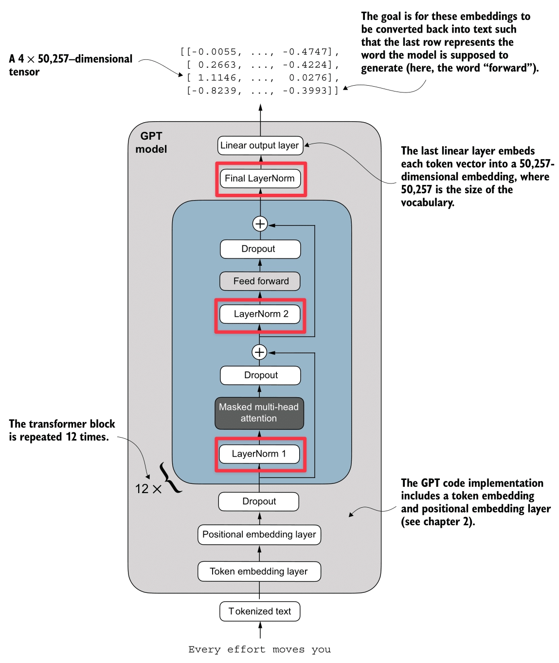
Layer Normalization stabilizes training and accelerates convergence by ensuring the inputs to a layer have a consistent distribution (Mean 0, Variance 1).
- Per-Token Normalization: Unlike Batch Normalization, Layer Norm is computed independently for each token (embedding vector). It calculates the mean and variance across the embedding dimension.
- Stability: It helps prevent Vanishing/Exploding Gradients and reduces Internal Covariate Shift (where the distribution of inputs to a layer changes during training).
- Learnable Parameters: After normalization, we apply a learnable Scale () and Shift (). This allows the model to “undo” the normalization if it helps the task, or adjust the distribution optimally.
Mathematical Definition
For a given input vector , Layer Normalization performs the following steps:
- Calculate Mean:
- Calculate Variance:
- Normalize:
- Output after Scale and Shift:
Where:
- is the dimension of the embedding.
- (epsilon) is a small constant to prevent division by zero.
- (scale) and (shift) are learnable parameters.
Simulation
Let’s walk through an example with real numbers. We’ll set a manual seed for reproducibility.
import torch

torch.manual_seed(123)
torch.set_printoptions(sci_mode=False)

# Imagine we have a batch of 2 inputs, each with an embedding dimension of 5
batch_example = torch.randn(2, 5)
print("Input:\n", batch_example)

# 1. Calculate Mean (across the last dimension)
mean = batch_example.mean(dim=-1, keepdim=True)
print("\nMean:\n", mean)

# 2. Calculate Variance (across the last dimension)
# Note: We use unbiased=False to match GPT-2's implementation style (dividing by N, not N-1)
var = batch_example.var(dim=-1, keepdim=True, unbiased=False)
print("\nVariance:\n", var)

# 3. Normalize
epsilon = 1e-5
normalized = (batch_example - mean) / torch.sqrt(var + epsilon)
print("\nNormalized:\n", normalized)

# Verify Mean is approx 0 and Variance is approx 1
print("\nMean of normalized:", normalized.mean(dim=-1))
print("Var of normalized:", normalized.var(dim=-1, unbiased=False))
Output:
Input:
 tensor([[-0.1115,  0.1204, -0.3696, -0.2404, -1.1969],
        [ 0.2093, -0.9724, -0.7550,  0.3239, -0.1085]])

Mean:
 tensor([[-0.3596],
        [-0.2606]])

Variance:
 tensor([[0.2015],
        [0.2673]])

Normalized:
 tensor([[ 0.5528,  1.0693, -0.0223,  0.2656, -1.8654],
        [ 0.9087, -1.3767, -0.9564,  1.1304,  0.2940]])

Mean of normalized: tensor([-0.0000,  0.0000])
Var of normalized: tensor([1.0000, 1.0000])
Why Epsilon?
Imagine an input vector where all elements are identical, e.g., .
- Calculate Mean:
- Calculate Variance:
- Normalize (Without ): . This results in a division by zero error or NaN (Not a Number).
- Normalize (With ): . This keeps the calculation mathematically stable.
Why Scale and Shift?
Normalization forces the inputs to a standard distribution (mean 0, variance 1). Sometimes, this might be too restrictive for the network. The learnable parameters (gamma) and (beta) give the model the flexibility to:
- Restore the original distribution if needed.
- Shift and scale the data to a range that is optimal for the next layer.
Example: If a normalized value is , and the network learns and : Without these parameters, the value would be stuck at 0.5.
Implementation
class LayerNorm(nn.Module):
def __init__(self, emb_dim):
super().__init__()
self.eps = 1e-5
self.scale = nn.Parameter(torch.ones(emb_dim))
self.shift = nn.Parameter(torch.zeros(emb_dim))
def forward(self, x):
mean = x.mean(dim=-1, keepdim=True)
var = x.var(dim=-1, keepdim=True, unbiased=False)
norm_x = (x - mean) / torch.sqrt(var + self.eps)
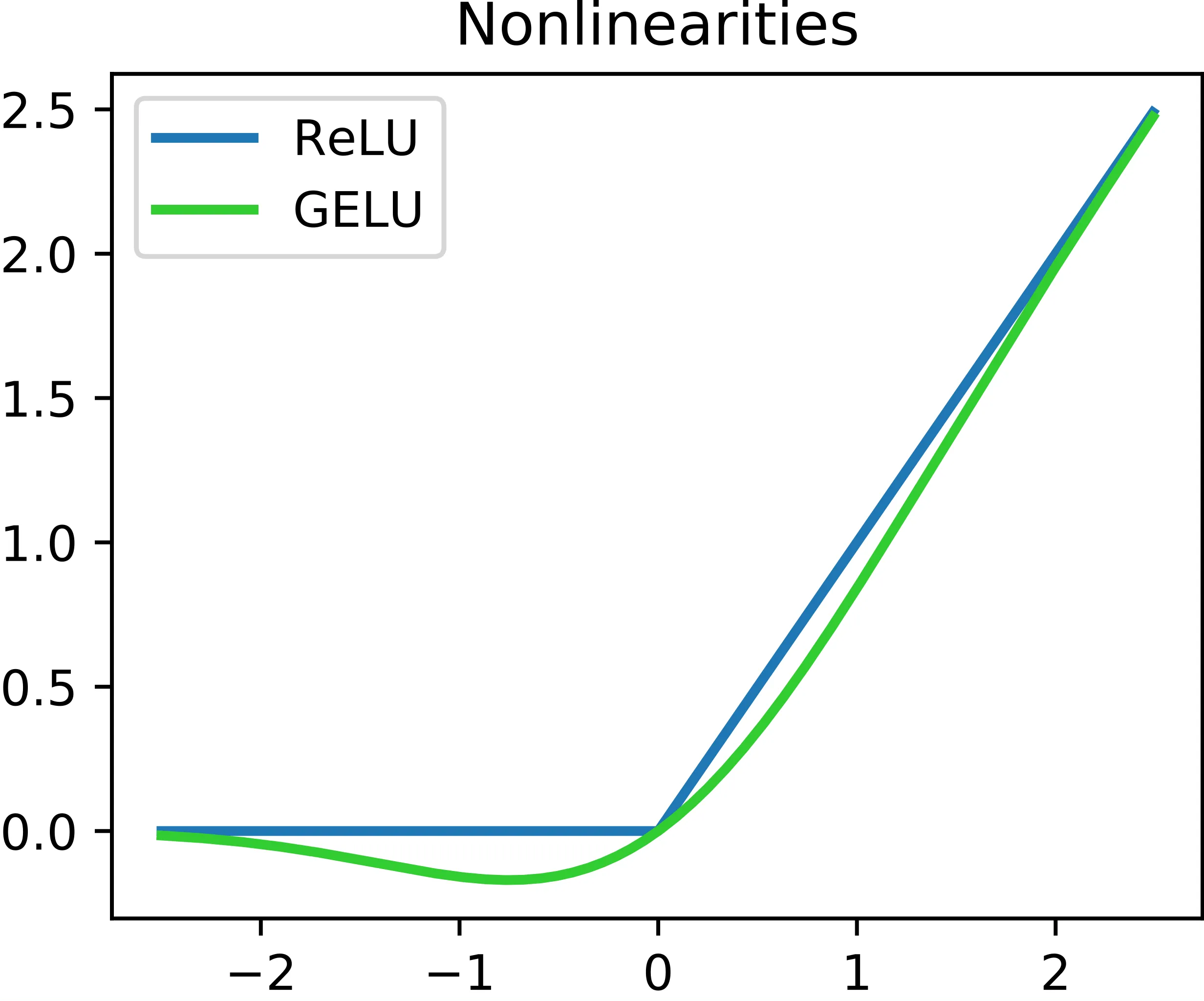
return self.scale * norm_x + self.shiftGELU (Gaussian Error Linear Unit)
Here’s the GELU process (highlighted in red):
The GELU activation function is defined as , where is the standard Gaussian Cumulative Distribution Function (CDF).
Why not ReLU?
- ReLU (Rectified Linear Unit) returns if positive, and if negative. It suffers from the Dead ReLU Problem, where neurons receiving negative inputs stop learning entirely because their gradients become zero.
- GELU addresses this by being smooth (differentiable everywhere) and allowing small negative values.
Key Advantages:
- Smoothness: Unlike ReLU’s sharp corner at 0, GELU is a smooth curve, leading to better optimization.
- No Dead Neurons: It prevents neurons from dying by allowing non-zero gradients for negative inputs.
In GPT-2, a tanh approximation is used for efficiency:
Implementation
class GELU(nn.Module):
    def __init__(self):
        super().__init__()

    def forward(self, x):
        return 0.5 * x * (1 + torch.tanh(
            torch.sqrt(torch.tensor(2.0 / torch.pi)) *
            (x + 0.044715 * torch.pow(x, 3))
        ))
Feed Forward Network (FFN)
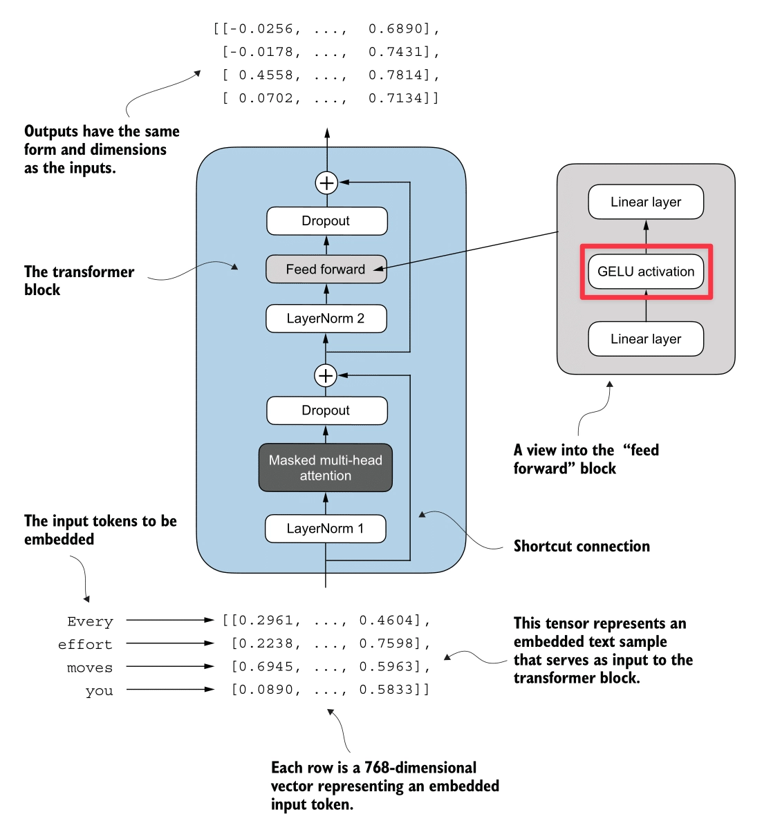
Here’s the Feed Forward Network process (highlighted in red):
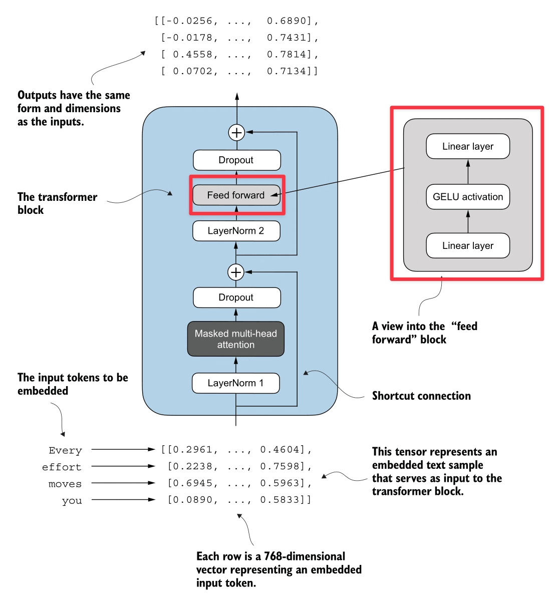
The Feed Forward Network applies a two-layer linear transformation to each token independently. Unlike Attention, which mixes information between tokens, the FFN processes information within each token’s embedding.
Expansion-Contraction Architecture
- Expansion: The input (embedding dimension ) is projected to a higher dimension ().
- For GPT-2 (124M), this is .
- Activation: The GELU activation is applied.
- Contraction: The vector is projected back to the original dimension ().
Why expand?
Moving to a higher-dimensional space allows the model to learn richer, more complex feature representations before compressing the information back into the embedding stream.
Implementation
class FeedForward(nn.Module):
    def __init__(self, cfg):
        super().__init__()
        self.layers = nn.Sequential(
            nn.Linear(cfg["emb_dim"], 4 * cfg["emb_dim"]), ## Expansion
            GELU(), ## Activation
            nn.Linear(4 * cfg["emb_dim"], cfg["emb_dim"]), ## Contraction
        )

    def forward(self, x):
        return self.layers(x)
Shortcut Connection
Here’s the Shortcut Connection process (highlighted in red):

Also known as Residual Connections or Skip Connections.
A Shortcut Connection simply adds the input of a layer to its output:
This creates an alternate path for the data to flow, bypassing the layer’s transformation.
The Vanishing Gradient Problem
In deep networks, gradients are calculated using the Chain Rule, which involves multiplying many small numbers together. As we go deeper (backwards from loss to input), these gradients can shrink exponentially—vanishing to zero. When this happens, the early layers stop learning.
How Shortcut Connections Help: They create a “Gradient Superhighway”. The gradient of is . That ensures that even if is tiny, the gradient can still flow back to earlier layers unchanged.
Simulation
We ran a simulation comparing a 5-layer network without and with shortcut connections to see the gradients (mean absolute value) at each layer.
class ExampleDeepNeuralNetwork(nn.Module):
    def __init__(self, layer_sizes, use_shortcut):
        super().__init__()
        self.use_shortcut = use_shortcut
        self.layers = nn.ModuleList([
            nn.Sequential(nn.Linear(layer_sizes[0], layer_sizes[1]), GELU()),
            nn.Sequential(nn.Linear(layer_sizes[1], layer_sizes[2]), GELU()),
            nn.Sequential(nn.Linear(layer_sizes[2], layer_sizes[3]), GELU()),
            nn.Sequential(nn.Linear(layer_sizes[3], layer_sizes[4]), GELU()),
            nn.Sequential(nn.Linear(layer_sizes[4], layer_sizes[5]), GELU())
        ])

    def forward(self, x):
        for layer in self.layers:
            layer_output = layer(x)
            if self.use_shortcut and x.shape == layer_output.shape:
                x = x + layer_output
            else:
                x = layer_output
        return x

def print_gradients(model, x):
    output = model(x)
    loss = nn.MSELoss()(output, torch.tensor([[0.]]))
    loss.backward()
    for name, param in model.named_parameters():
        if 'weight' in name:
            print(f"{name} has gradient mean of {param.grad.abs().mean().item()}")
Output:
--- Model WITHOUT Shortcut Connections ---
layers.0.0.weight has gradient mean of 0.00020173587836325169
layers.1.0.weight has gradient mean of 0.0001201116101583466
layers.2.0.weight has gradient mean of 0.0007152041071094573
layers.3.0.weight has gradient mean of 0.0013988735154271126
layers.4.0.weight has gradient mean of 0.005049645435065031

--- Model WITH Shortcut Connections ---
layers.0.0.weight has gradient mean of 0.22169791162014008
layers.1.0.weight has gradient mean of 0.20694106817245483
layers.2.0.weight has gradient mean of 0.32896995544433594
layers.3.0.weight has gradient mean of 0.2665732204914093
layers.4.0.weight has gradient mean of 1.3258540630340576
Observation:
- Without Shortcuts: The gradient vanishes from 0.005 (Layer 4) down to 0.0002 (Layer 0).
- With Shortcuts: The gradients remain strong and consistent across all layers.
Implementation
The key is adding the input x back to the output layer_output.
## Example Logic
for layer in self.layers:
    layer_output = layer(x)
    if self.use_shortcut:
        x = x + layer_output ## The Shortcut
    else:
        x = layer_output
Transformer Block
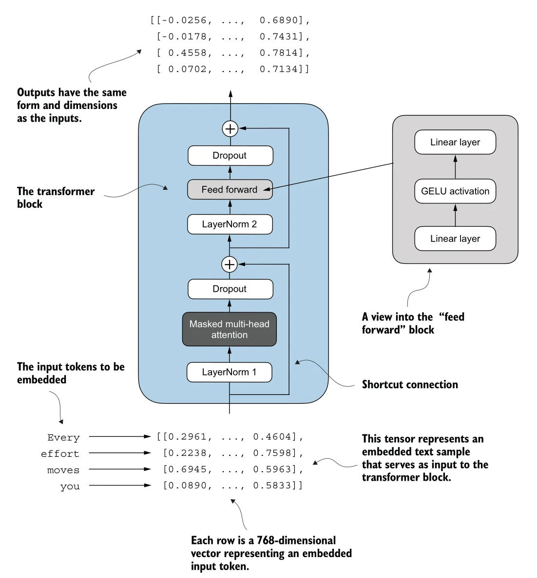
Finally, here’s the Transformer block (highlighted in red):
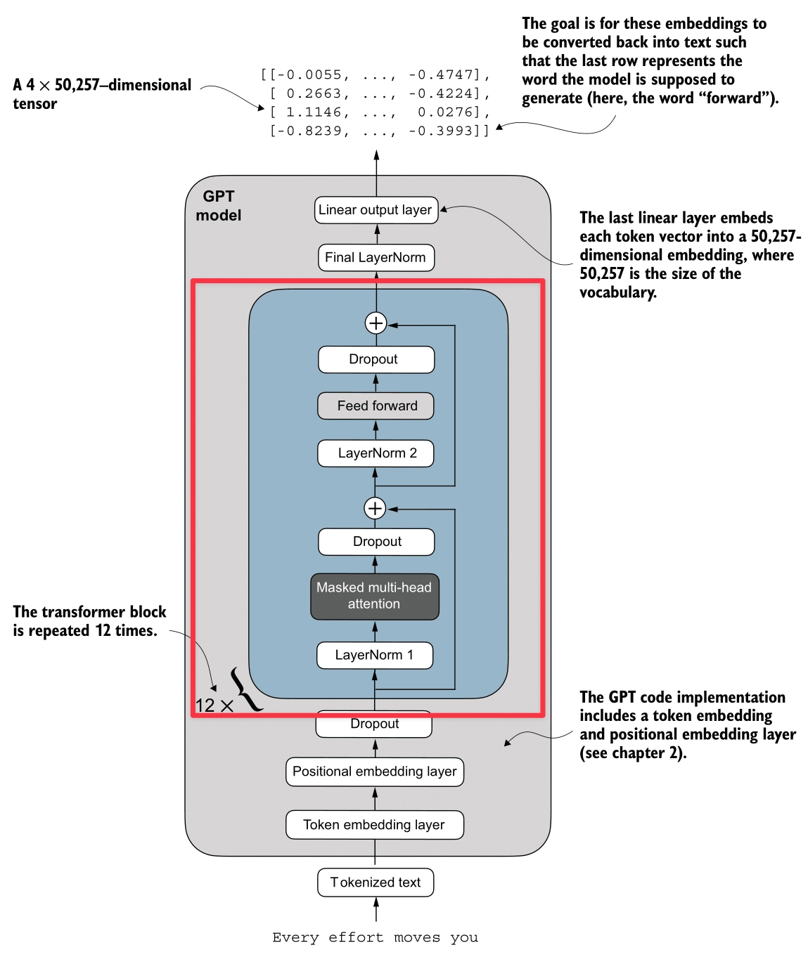
We assemble all the components into the Transformer Block. This is the fundamental repeating unit of the GPT architecture.
Pre-LayerNorm Architecture
The GPT model uses a Pre-LayerNorm design, which is more stable for training deep networks than the original Post-LayerNorm.
The Logic Flow:
- Input
- Attention Path:
- Normalize :
x_norm = LayerNorm(x) - Compute Attention:
attn = MultiHeadAttention(x_norm) - Apply Dropout:
attn = Dropout(attn) - Shortcut: Add back to original input:
x = x + attn
- Normalize :
- Feed Forward Path:
- Normalize :
x_norm = LayerNorm(x) - Compute Feed Forward:
ffn = FeedForward(x_norm) - Apply Dropout:
ffn = Dropout(ffn) - Shortcut: Add back to input:
x = x + ffn
- Normalize :
Shape Preservation
A crucial property of the Transformer Block is that it preserves dimensions.
- Input: (e.g., )
- Output: (e.g., )
This allows us to stack these blocks essentially endlessly (12 stacks for GPT-2 Small, 96 stacks for GPT-3).
Implementation
class TransformerBlock(nn.Module):
    def __init__(self, cfg):
        super().__init__()
        self.att = MultiHeadAttention(
            d_in=cfg["emb_dim"],
            d_out=cfg["emb_dim"],
            context_length=cfg["context_length"],
            num_heads=cfg["n_heads"],
            dropout=cfg["drop_rate"],
            qkv_bias=cfg["qkv_bias"])
        self.ff = FeedForward(cfg)
        self.norm1 = LayerNorm(cfg["emb_dim"])
        self.norm2 = LayerNorm(cfg["emb_dim"])
        self.drop_shortcut = nn.Dropout(cfg["drop_rate"])

    def forward(self, x):
        # 1. Attention Block with Shortcut
        shortcut = x
        x = self.norm1(x)
        x = self.att(x)  # Shape [batch_size, num_tokens, emb_size]
        x = self.drop_shortcut(x)
        x = x + shortcut  # Add the original input back

        # 2. Feed Forward Block with Shortcut
        shortcut = x
        x = self.norm2(x)
        x = self.ff(x)
        x = self.drop_shortcut(x)
        x = x + shortcut  # Add the original input back

        return x
2. Code the entire GPT Model
We now have all the building blocks to assemble the full GPT architecture.
We will use the configuration for GPT-2 Small (124 Million Parameters):
- Vocab Size: 50,257 (OpenAI’s BPE Tokenizer)
- Context Length: 1024 tokens
- Embedding Dimension: 768
- Number of Attention Heads: 12
- Number of Transformer Blocks: 12
- Dropout Rate: 0.1
- Query-Key-Value Bias: True (GPT-2 uses QKV bias, but modern LLMs usually don’t)
GPT Model Class
The GPTModel class orchestrates the entire flow:
- Embeddings: Converts token IDs to semantic vectors + adds positional info.
- Transformer Stack: Passes input through 12 Transformer Blocks.
- Head: Normalizes and projects back to vocabulary logits.
GPT_CONFIG_124M = {
    "vocab_size": 50257,    # Vocabulary size
    "context_length": 1024, # Context length
    "emb_dim": 768,         # Embedding dimension
    "n_heads": 12,          # Number of attention heads
    "n_layers": 12,         # Number of transformer blocks
    "drop_rate": 0.1,       # Dropout rate
    "qkv_bias": True        # Query-Key-Value bias
}

class GPTModel(nn.Module):
    def __init__(self, cfg):
        super().__init__()
        # 1. Embeddings
        self.tok_emb = nn.Embedding(cfg["vocab_size"], cfg["emb_dim"])
        self.pos_emb = nn.Embedding(cfg["context_length"], cfg["emb_dim"])
        self.drop_emb = nn.Dropout(cfg["drop_rate"])

        # 2. Transformer Blocks Stack
        self.trf_blocks = nn.Sequential(
            *[TransformerBlock(cfg) for _ in range(cfg["n_layers"])])

        # 3. Final Norm & Output Head
        self.final_norm = LayerNorm(cfg["emb_dim"])
        self.out_head = nn.Linear(
            cfg["emb_dim"], cfg["vocab_size"], bias=False
        )

    def forward(self, in_idx):
        batch_size, seq_len = in_idx.shape

        # Input Embeddings
        tok_embeds = self.tok_emb(in_idx)
        pos_embeds = self.pos_emb(torch.arange(seq_len, device=in_idx.device))
        x = tok_embeds + pos_embeds
        x = self.drop_emb(x)

        # Transformer Blocks
        x = self.trf_blocks(x)

        # Output Head
        x = self.final_norm(x)
        logits = self.out_head(x)

        return logits
3. Pre-Training
To train our GPT model, we need to measure how “wrong” its predictions are and update the weights to improve them. We use Cross Entropy Loss for this.
1. Calculating Loss
For every input sequence, the “Target” (the true label) is simply the input shifted by one position. This is often called “Teacher Forcing”.
- Input:
Every effort moves you - Target:
effort moves you [NextWord]
We compute the loss for a batch of data:
def calc_loss_batch(input_batch, target_batch, model, device):
    input_batch = input_batch.to(device)
    target_batch = target_batch.to(device)

    # 1. Forward Pass: Get Logits
    logits = model(input_batch)

    # 2. Flatten for CrossEntropyLoss
    # Logits shape: [batch * context_len, vocab_size]
    # Targets shape: [batch * context_len]
    loss = nn.functional.cross_entropy(
        logits.flatten(0, 1),
        target_batch.flatten()
    )
    return loss
2. Training Loop
We use the standard PyTorch training loop with the AdamW optimizer.
For each batch:
- Forward Pass: Compute loss.
- Backward Pass: Calculate gradients (
loss.backward()). - Update: Update weights (
optimizer.step()). - Reset: Clear gradients (
optimizer.zero_grad()).
def train_model(model, train_loader, val_loader, optimizer, device, num_epochs,
                       eval_freq, eval_iter):
    train_losses, val_losses, track_tokens_seen = [], [], []
    tokens_seen, global_step = 0, -1

    for epoch in range(num_epochs):
        model.train() # Set to training mode

        for input_batch, target_batch in train_loader:
            optimizer.zero_grad() # Reset gradients

            # Forward + Backward + Update
            loss = calc_loss_batch(input_batch, target_batch, model, device)
            loss.backward()       # Calculate gradients
            optimizer.step()      # Update weights

            tokens_seen += input_batch.numel()
            global_step += 1

            # Optional: Evaluate every specific steps
            if global_step % eval_freq == 0:
                print(f"Ep {epoch+1} (Step {global_step:06d}): "
                      f"Train loss {loss.item():.3f}")

    return train_losses, val_losses
Result:
Train loader len: 4
Val loader len: 1
Starting training...
Ep 1 (Step 000000): Train loss 9.865, Val loss 9.905
Every effort moves you, the, the the the, the, the the the the the the the, the the the, the the the the the the, the the, the the the, the the the the the the the, the the, the, the the
Ep 2 (Step 000005): Train loss 7.761, Val loss 8.084
Every effort moves you,,,,,,,,,,,,,,,,,,,,,,,,,,,,,,,,,,,,,,,,,,,,,,,,,,
Ep 3 (Step 000010): Train loss 6.259, Val loss 6.847
Every effort moves you, and, and the the, and, and the, and the, and, and the, and, and, and the, and the the, and the, and the, and the, and the, and the, and, and the
Ep 4 (Step 000015): Train loss 5.418, Val loss 6.373
Every effort moves you, I had the a the a--I had the--I--I had the, and I had a--I had the--I had the, and I had a, and had the--I had, and had the--I had a
Every effort moves you in the to have a little of the first to have a little me--I had been of the picture--I had been of theI.
Ep 6 (Step 000020): Train loss 4.368, Val loss 6.338
Every effort moves you know the fact--as the picture--as he had been. "--and, with a, and Mrs. "--and, with a little a little, and I had been's he had been, and, and he was his
Ep 7 (Step 000025): Train loss 2.999, Val loss 6.172
Every effort moves you know the fact--his the picture--and I felt--as me--and I felt--and I had been I had been to have been I had been his pictures--and that, and I had been his pictures--and that he had been
Ep 8 (Step 000030): Train loss 2.922, Val loss 6.169
Every effort moves you know he was one of the picture--I--I had been the Sev I had been his pictures, and Mrs. "I turned, I had been his pictures--his.   "I had been; and Mrs.
Ep 9 (Step 000035): Train loss 2.408, Val loss 6.183
Every effort moves you know," was one of the one of the to the fact with the Sev I had been his own's an!     "I turned back the donkey-c--as one had to the donkey. "There were, I had
Every effort moves you in the inevitable garlanded to have to the that he had the Sevres and I had been's an!     "I turned back the _rose, and; and I had the, and down the room, and I
Observation: Overfitting
If you look closely at the logs, you’ll see a classic sign of overfitting:
- Validation Loss Stagnation: The validation loss stops decreasing (around
6.1) while the training loss keeps dropping (to2.4). - Memorization: The model starts regurgitating exact phrases from the training data. For example, “Sevres”, “donkey”, and “picture” are specific words from the training data:
the-verdict.txt.
This happens because our model is very large (124M parameters) relative to our tiny dataset. In a real-world scenario, we would need a massive dataset (billions of tokens) to prevent this and learn generalizable patterns.
4. Text Generation
Autoregressive Prediction
GPT generates text autoregressively: it predicts one token at a time, and “eats” its own output as the input for the next step.
- Input: “Every effort moves”
- Model: Predicts ” you”
- New Input: “Every effort moves you”
- Model: Predicts ” forward”
Here is a simple loop to achieve this:
def generate_text(model, idx, max_new_tokens, context_size):
    for _ in range(max_new_tokens):
        # 1. Crop context to context window size
        idx_cond = idx[:, -context_size:]

        # 2. Get predictions
        with torch.no_grad():
            logits = model(idx_cond)

        # 3. Focus on last step (next token prediction)
        logits = logits[:, -1, :]
        probs = torch.softmax(logits, dim=-1)

        # 4. Get most likely token (Greedy)
        idx_next = torch.argmax(probs, dim=-1, keepdim=True)

        # 5. Append to context
        idx = torch.cat((idx, idx_next), dim=1)
    return idx
Result:
Input: 'Every effort moves you'
Output: 'Every effort moves you in the inevitable garlanded to have to the that he had the Sevres and I had been's an!


"I turned back the _rose, and; and I had the, and down the room, and I'
(Note: As we saw earlier, the model has overfit. It’s repeating “Sevres” and “garlanded” from the training text, essentially reciting the book instead of generating new creative text.)
Avoid Greedy Decoding
The simplest way to generate text is Greedy Decoding: always picking the token with the highest probability (argmax).
idx_next = torch.argmax(logits, dim=-1, keepdim=True)But this often leads to repetitive and boring text. It also prevents the model from correcting itself if it makes a suboptimal choice early on (it can’t “backtrack”).
Temperature
To fix this, we sample from the probability distribution instead of just taking the max. Temperature () scales the logits before the Softmax.
- High (> 1.0): Flattens the distribution. Rare words become more likely (More creative/random).
- Low (< 1.0): Sharpens the distribution. The most likely words become even more likely (More confident/conservative).
logits = logits / temperature
probs = torch.softmax(logits, dim=-1)
idx_next = torch.multinomial(probs, num_samples=1)
Top K Sampling
Even with temperature, there’s a risk of sampling a very incorrect word from the “long tail” of the distribution (e.g., “The cat sat on the… pizza”).
Top-K Sampling fixes this by:
- Selecting the top most likely tokens.
- Setting the probability of all other tokens to (or zero).
- Re-normalizing and sampling from this filtered set.
This ensures we only choose from “reasonable” options while still maintaining variety.
if top_k is not None:
    top_logits, _ = torch.topk(logits, top_k)
    min_val = top_logits[:, -1]
    # Mask logits below the top-k threshold
    logits = torch.where(logits < min_val, torch.tensor(float("-inf")).to(logits.device), logits)
Implementation
Here is the complete generation function combining all these strategies:
def generate(model, idx, max_new_tokens, context_size, temperature=0.0, top_k=None, eos_id=None):
    for _ in range(max_new_tokens):
        # crop current context to context_size
        idx_cond = idx[:, -context_size:]

        with torch.no_grad():
            logits = model(idx_cond)

        # focus only on the last time step
        logits = logits[:, -1, :]

        if top_k is not None:
            top_logits, _ = torch.topk(logits, top_k)
            min_val = top_logits[:, -1]
            logits = torch.where(logits < min_val, torch.tensor(float("-inf")).to(logits.device), logits)

        if temperature > 0.0:
            logits = logits / temperature
            probs = torch.softmax(logits, dim=-1)
            idx_next = torch.multinomial(probs, num_samples=1)
        else:
            idx_next = torch.argmax(logits, dim=-1, keepdim=True)

        if idx_next == eos_id:
            break

        idx = torch.cat((idx, idx_next), dim=1)
    return idx
5. Load Pre-Trained Weights from OpenAI GPT-2
Training a LLM from scratch requires massive computing costs. Fortunately, we can load the pre-trained weights from OpenAI’s GPT-2 (124M parameters) into our architecture.
Kaggle OpenAI gpt-2 weights: OpenAI GPT-2 Weights
Parameter Mapping
OpenAI’s implementation (TensorFlow) uses different variable names than our PyTorch implementation. We need to map them carefully.
| OpenAI Name | Our Name | Description |
|---|---|---|
wte | tok_emb | Token Embeddings |
wpe | pos_emb | Positional Embeddings |
ln_1, ln_2 | norm1, norm2 | Layer Norms |
mlp.c_fc, mlp.c_proj | ff.layers[0], ff.layers[2] | Feed Forward Layers |
attn.c_attn | W_query, W_key, W_value | Attention Weights (Fused in OpenAI) |
Loading Logic
First, we need the assign helper to ensure shapes match:
def assign(left, right):
    if left.shape != right.shape:
        raise ValueError(f"Shape mismatch. Left: {left.shape}, Right: {right.shape}")
    return torch.nn.Parameter(torch.tensor(right))
Then, the main loading function:
import numpy as np

def load_weights_into_gpt(gpt, params):
    gpt.pos_emb.weight = assign(gpt.pos_emb.weight, params['wpe'])
    gpt.tok_emb.weight = assign(gpt.tok_emb.weight, params['wte'])

    for b in range(len(params["blocks"])):
        # 1. Attention Weights (Split q, k, v)
        q_w, k_w, v_w = np.split(
            (params["blocks"][b]["attn"]["c_attn"])["w"], 3, axis=-1)
        gpt.trf_blocks[b].att.W_query.weight = assign(gpt.trf_blocks[b].att.W_query.weight, q_w.T)
        gpt.trf_blocks[b].att.W_key.weight = assign(gpt.trf_blocks[b].att.W_key.weight, k_w.T)
        gpt.trf_blocks[b].att.W_value.weight = assign(gpt.trf_blocks[b].att.W_value.weight, v_w.T)

        # 2. Attention Biases (Split q, k, v)
        q_b, k_b, v_b = np.split(
            (params["blocks"][b]["attn"]["c_attn"])["b"], 3, axis=-1)
        gpt.trf_blocks[b].att.W_query.bias = assign(gpt.trf_blocks[b].att.W_query.bias, q_b)
        gpt.trf_blocks[b].att.W_key.bias = assign(gpt.trf_blocks[b].att.W_key.bias, k_b)
        gpt.trf_blocks[b].att.W_value.bias = assign(gpt.trf_blocks[b].att.W_value.bias, v_b)

        # 3. Attention Output Projection
        gpt.trf_blocks[b].att.out_proj.weight = assign(
            gpt.trf_blocks[b].att.out_proj.weight,
            params["blocks"][b]["attn"]["c_proj"]["w"].T)
        gpt.trf_blocks[b].att.out_proj.bias = assign(
            gpt.trf_blocks[b].att.out_proj.bias,
            params["blocks"][b]["attn"]["c_proj"]["b"])

        # 4. Feed Forward Weights
        gpt.trf_blocks[b].ff.layers[0].weight = assign(
            gpt.trf_blocks[b].ff.layers[0].weight,
            params["blocks"][b]["mlp"]["c_fc"]["w"].T)
        gpt.trf_blocks[b].ff.layers[0].bias = assign(
            gpt.trf_blocks[b].ff.layers[0].bias,
            params["blocks"][b]["mlp"]["c_fc"]["b"])
        gpt.trf_blocks[b].ff.layers[2].weight = assign(
            gpt.trf_blocks[b].ff.layers[2].weight,
            params["blocks"][b]["mlp"]["c_proj"]["w"].T)
        gpt.trf_blocks[b].ff.layers[2].bias = assign(
            gpt.trf_blocks[b].ff.layers[2].bias,
            params["blocks"][b]["mlp"]["c_proj"]["b"])

        # 5. Layer Norms
        gpt.trf_blocks[b].norm1.scale = assign(
            gpt.trf_blocks[b].norm1.scale,
            params["blocks"][b]["ln_1"]["g"])
        gpt.trf_blocks[b].norm1.shift = assign(
            gpt.trf_blocks[b].norm1.shift,
            params["blocks"][b]["ln_1"]["b"])
        gpt.trf_blocks[b].norm2.scale = assign(
            gpt.trf_blocks[b].norm2.scale,
            params["blocks"][b]["ln_2"]["g"])
        gpt.trf_blocks[b].norm2.shift = assign(
            gpt.trf_blocks[b].norm2.shift,
            params["blocks"][b]["ln_2"]["b"])

    # 6. Final Layer Norm & Output Head
    gpt.final_norm.scale = assign(gpt.final_norm.scale, params["g"])
    gpt.final_norm.shift = assign(gpt.final_norm.shift, params["b"])
gpt.out_head.weight = assign(gpt.out_head.weight, params["wte"])Note: The .T (transpose) is necessary because TensorFlow stores weights as (in, out) while PyTorch stores them as (out, in).
Text Generation
Once loaded, the model generates coherent English text:
uv run ./generate.py "Every effort moves you" --max_tokens 30 --temperature 0.5 --top_k 3
Generating text for prompt: 'Every effort moves you'

--- Generated Text ---
Every effort moves you to the next level and you are rewarded with a higher level of success.

The best part is that you can do all this without spending a
uv run ./generate.py "Every effort moves you" --max_tokens 50 --temperature 0.5 --top_k 3
Generating text for prompt: 'Every effort moves you'
--- Generated Text ---
Every effort moves you to the next step.
The first step is to get your mind on the right track.
You need to know how to get your mind on the right track.
The second step is to get your mind on the right track