Neural Network Backbone

1. Neuron

A Neuron is the fundamental atomic unit. It takes multiple inputs ( $x$ ), multiplies each by a distinct weight ( $w$ ), and sums them up. Finally, it adds a bias ( $b$ ) to this sum. This linear operation allows the neuron to “weigh” the importance of different inputs.

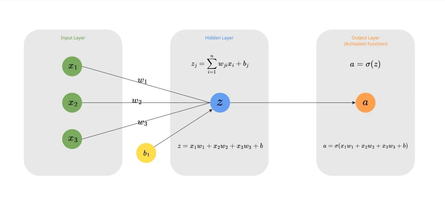
For the single neuron above with 3 inputs, the calculation is:

\text{Output} = x_1 w_1 + x_2 w_2 + x_3 w_3 + b

Real power comes when we stack these neurons together into a Layer. This allows the network to learn multiple different features from the same input data simultaneously.

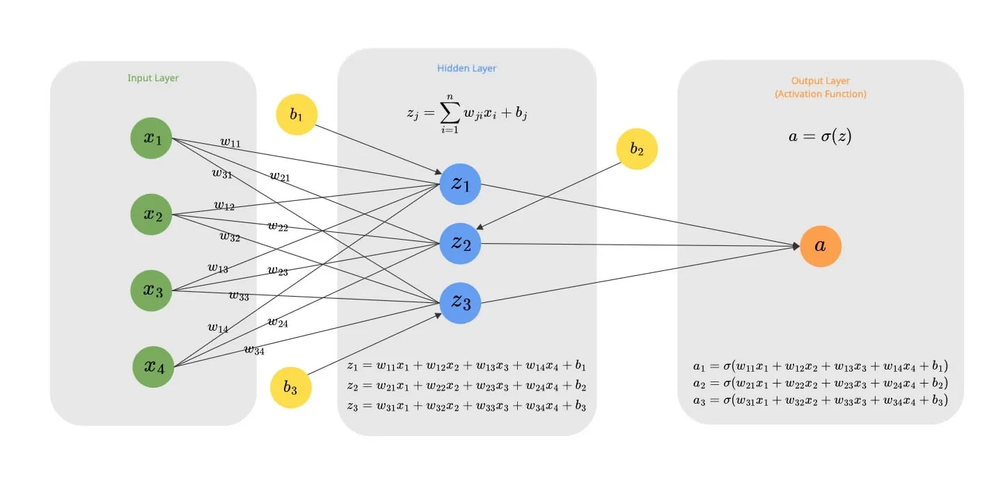
Consider a layer of 3 neurons receiving 4 inputs ( $x_1, x_2, x_3, x_4$ ). Each neuron maintains its own unique set of weights and its own bias:

Neuron 1: $z_1 = w_{11}x_1 + w_{12}x_2 + w_{13}x_3 + w_{14}x_4 + b_1$
Neuron 2: $z_2 = w_{21}x_1 + w_{22}x_2 + w_{23}x_3 + w_{24}x_4 + b_2$
Neuron 3: $z_3 = w_{31}x_1 + w_{32}x_2 + w_{33}x_3 + w_{34}x_4 + b_3$

We can generalize this calculation for any neuron $j$ as:

z_j = \sum_{i=1}^{n} w_{ji} x_i + b_j

Dot Product

This operation of multiplying elements and summing them up ( $x_1 w_1 + \dots$ ) is mathematically known as the Dot Product.

\text{Input} \cdot \text{Weight} = \sum (x_i \cdot w_i)

So, we can rewrite our neuron’s output formula more compactly as:

z = \mathbf{w} \cdot \mathbf{x} + b

Python Code Example

2. Activation Function

The output we calculated above ( $z = wx+b$ ) is purely linear.

Here is the problem: Stacking multiple linear layers is mathematically equivalent to just one big linear layer. No matter how deep you make your network, if it’s all linear, it can only learn straight lines. It cannot capture complex patterns like curves or shapes.

To solve this, we introduce non-linearity by passing the output $z$ through an Activation Function.

Rectified Linear Unit (ReLU)

The most basic choice for hidden layers is ReLU (Rectified Linear Unit).

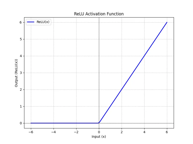
It essentially says: “If the value is positive, keep it. If it’s negative, make it zero.”

a = ReLU(z) = \max(0, z)

If we apply this to our neurons, we do it element-wise.

a_j = ReLU(z_j) = \max(0, \sum_{i} w_{ji} x_i + b_j)

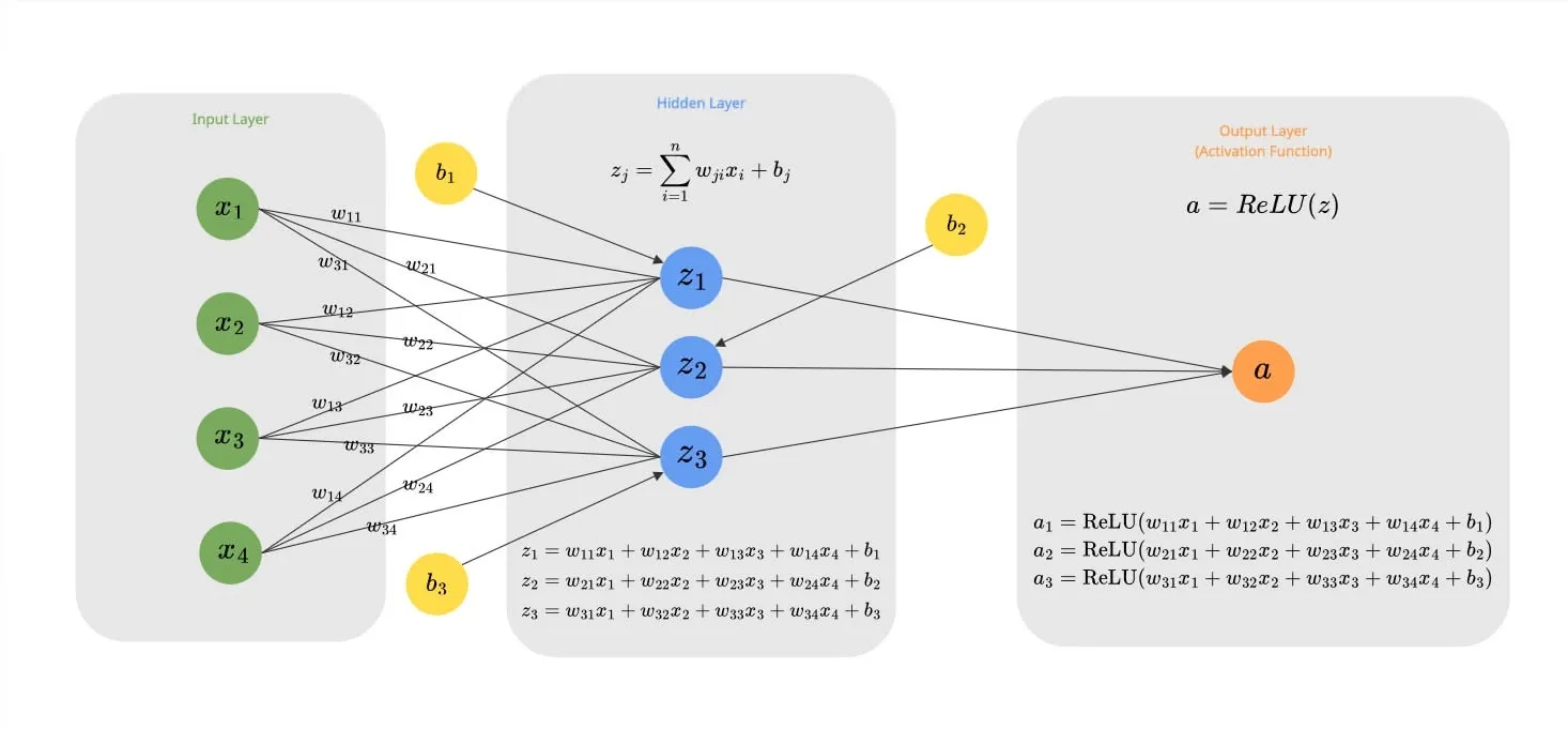
In case of the above example with 3 neurons:

\begin{aligned} a_1 &= \max(0, z_1) \\ a_2 &= \max(0, z_2) \\ a_3 &= \max(0, z_3) \end{aligned}

Python Code Example of ReLU

Result:

--- NumPy Implementation ---
Weights (4x3):
 [[ 0.04967142 -0.01382643  0.06476885]
 [ 0.15230299 -0.02341534 -0.0234137 ]
 [ 0.15792128  0.07674347 -0.04694744]
 [ 0.054256   -0.04634177 -0.04657298]]
Biases (1x3):
 [[0. 0. 0.]]
Linear Output (z):
 [[ 0.96368124  0.05371889 -0.23933329]]
Activated Output (a = ReLU(z)):
 [[0.96368124 0.05371889 0.        ]]

--- PyTorch Implementation ---
Weights (4x3):
 [[ 0.04967142 -0.01382643  0.06476885]
 [ 0.15230298 -0.02341534 -0.0234137 ]
 [ 0.15792128  0.07674348 -0.04694744]
 [ 0.054256   -0.04634177 -0.04657298]]
Biases (1x3):
 [0. 0. 0.]
Linear Output (z):
 [[ 0.9636813   0.05371889 -0.2393333 ]]
Activated Output (a = ReLU(z)):
 [[0.9636813  0.05371889 0.        ]]

Softmax

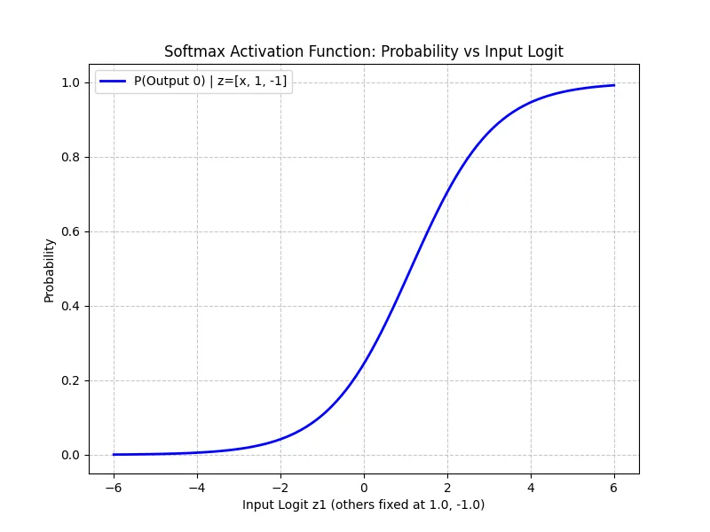
For the final output layer, especially in classification tasks (like predicting the next token in a LLM), we want probabilities. We want to know: “What is the % chance that this token is Next?”

Softmax function takes raw numbers (logits) and converts them into a probability distribution summing to 1.

\text{Softmax}(z_i) = \frac{e^{z_i}}{\sum_{j} e^{z_j}}

Python Code Example of Softmax

Result:

--- NumPy Implementation ---
Weights (4x3):
 [[ 0.04967142 -0.01382643  0.06476885]
 [ 0.15230299 -0.02341534 -0.0234137 ]
 [ 0.15792128  0.07674347 -0.04694744]
 [ 0.054256   -0.04634177 -0.04657298]]
Biases (1x3):
 [[0. 0. 0.]]
Linear Output (logits):
 [[ 0.96368124  0.05371889 -0.23933329]]
Final Output (Probabilities):
 [[0.58725872 0.23639476 0.17634652]]
Sum of probabilities:  1.0

--- PyTorch Implementation ---
Weights (4x3):
 [[ 0.04967142 -0.01382643  0.06476885]
 [ 0.15230298 -0.02341534 -0.0234137 ]
 [ 0.15792128  0.07674348 -0.04694744]
 [ 0.054256   -0.04634177 -0.04657298]]
Biases (1x3):
 [0. 0. 0.]
Linear Output (logits):
 [[ 0.9636813   0.05371889 -0.2393333 ]]
Final Output (Probabilities):
 [[0.5872587  0.23639473 0.17634651]]
Sum of probabilities:  1.0

3. Loss Function

How do we know if our neural network is doing a good job? We need a score to measure its performance. A Loss Function (or Cost Function) quantifies the error between the network’s prediction and the actual target.

Different tasks require different loss functions. Here, $\hat{y}$ represents the predicted value (our activation output $a$ ) and $y$ represents the true target.

Mean Absolute Error (MAE): often used for regression when outliers shouldn’t be penalized too heavily.

L = \frac{1}{n} \sum_{i=1}^{n} |y^{(i)} - \hat{y}^{(i)}|

Cross-Entropy Loss: The standard for classification tasks like image classification and also used for predicting the next token in GPT models.

L = -\frac{1}{n} \sum_{i=1}^{n} \sum_{c=1}^{C} y_{c}^{(i)} \log(\hat{y}_{c}^{(i)})

Python Code Example of MSE Loss

Let’s calculate the loss for this simple network example introduced in the previous section. We will use the Mean Squared Error (MSE) loss function.

Resule:

Inputs: [[1.0, 2.0, 3.0, 2.5]]
Target: [0.0, 0.0, 0.0]

--- NumPy Implementation ---
Prediction (a):
[[0.96368124 0.05371889 0.        ]]
MSE Loss:
0.31052241854349866

--- PyTorch Implementation ---
Prediction (a):
[[0.9636813  0.05371889 0.        ]]
PyTorch MSELoss:
0.3105224370956421

4. Backpropagation

This is the “engine” of learning. We just calculated the Loss ( $L$ ). Now we need to know: “How much did each weight contribute to this error?”

If we know that increasing weight $w_{11}$ by a tiny bit increases the error, then we should decrease $w_{11}$ . This “sensitivity” is called a Gradient.

We calculate these gradients using the Chain Rule of calculus, propagating the error backward from the output to the input.

\frac{dz}{dx} = \frac{dz}{dy} \cdot \frac{dy}{dx}

Let’s look at the simple network example that we saw above:

First, let’s calculate the loss function for the output $a$ :

\begin{aligned} L &= (a - \text{Target})^2 \\ &= (\text{ReLU}(\text{z}) - 0)^2 \\ &= \left( \text{ReLU} \left( \text{sum} \left( \begin{aligned} &\text{mul}(x_1, w_1), \text{mul}(x_2, w_2), \\ &\text{mul}(x_3, w_3), \text{mul}(x_4, w_4), b \end{aligned} \right) \right) \right)^2 \end{aligned}

(Note: In this specific example, we set the Target to 0 to simplify the math. We want the neuron to learn to output 0.)

To find the gradient of the Loss with respect to a specific weight (e.g., $w_{11}$ connecting Input 1 to Neuron 1), we use the chain rule. We trace the path from the Loss back to the weight:

Path: Loss $\rightarrow$ ReLU $\rightarrow$ Sum $\rightarrow$ Mul $\rightarrow$ $w_{11}$

\frac{\partial \text{Loss}}{\partial w_{11}} = \frac{\partial \text{Loss}}{\partial \text{ReLU}} \cdot \frac{\partial \text{ReLU}}{\partial \text{sum}} \cdot \frac{\partial \text{sum}}{\partial \text{mul}} \cdot \frac{\partial \text{mul}}{\partial w_{11}}

Using the values from our actual code execution (where $x_1=1.0$ , $z \approx 0.964$ , $a \approx 0.964$ ):

$\frac{\partial \text{Loss}}{\partial \text{ReLU}}$ : The derivative of Mean Squared Error ( $\frac{1}{n}\sum(a-y)^2$ $\frac{1}{n} \sum (a - y)^{2}$ ) with respect to $a$ $a$ . Since we have $n=3$ $n = 3$ neurons:
- Formula: $\frac{2}{3}(a - \text{Target})$
- Result: $\frac{2}{3}(0.964 - 0) \approx 0.642$
$\frac{\partial \text{ReLU}}{\partial \text{sum}}$ : Since $z (0.964) > 0$ , the slope is $1$ .
$\frac{\partial \text{sum}}{\partial \text{mul}}$ : $1$ .
$\frac{\partial \text{mul}}{\partial w_{11}}$ : Input $x_1 = 1.0$ .

Final Gradient for $w_{11}$ :

\frac{\partial \text{Loss}}{\partial w_{11}} = 0.642 \cdot 1 \cdot 1 \cdot 1.0 = 0.642

This positive gradient tells us that increasing $w_{11}$ will increase the error, so we should decrease it.

Python Code Example

Result:


--- NumPy Implementation (Manual Backprop) ---
Loss: 0.31052241854349866
Gradients (NumPy):
  dLoss/dW:
[[0.64245416 0.03581259 0.        ]
 [1.28490832 0.07162519 0.        ]
 [1.92736248 0.10743778 0.        ]
 [1.6061354  0.08953148 0.        ]]
  dLoss/db:
[[0.64245416 0.03581259 0.        ]]

--- PyTorch Implementation (AutoGrad) ---
Gradients (PyTorch):
  dLoss/dW:
[[0.6424542  0.0358126  0.        ]
 [1.2849084  0.0716252  0.        ]
 [1.9273627  0.10743779 0.        ]
 [1.6061355  0.0895315  0.        ]]
  dLoss/db:
[0.6424542 0.0358126 0.       ]

5. Gradient Descent

Now that we have the gradients (the “direction” of error), we can fix our weights.

We update the weights by moving them in the opposite direction of the gradient. We take a small step, determined by the Learning Rate ( $\alpha$ ).

w_{new} = w_{old} - \alpha \cdot \frac{\partial L}{\partial w}

By repeating this process (Forward Pass $\rightarrow$ Calculate Loss $\rightarrow$ Backprop $\rightarrow$ Gradient Descent) thousands of times, the weights slowly converge to the optimal values that solve the problem.

Python Code Example of Gradient Descent Loop

Result:

Start Weights:
[[ 0.04967142 -0.01382643  0.06476885]
 [ 0.15230299 -0.02341534 -0.0234137 ]
 [ 0.15792128  0.07674347 -0.04694744]
 [ 0.054256   -0.04634177 -0.04657298]]

Epoch 1: Loss = 0.3105, Grad Norm = 2.8955
  Gradient (dLoss/dW):
[[0.6425 0.0358 0.    ]
 [1.2849 0.0716 0.    ]
 [1.9274 0.1074 0.    ]
 [1.6061 0.0895 0.    ]]
  Weight Update (Old - Step = New):
  Old Weights               Step (LR*Grad)            New Weights
  [ 0.0497 -0.0138  0.0648] - [0.0064 0.0004 0.    ]    = [ 0.0432 -0.0142  0.0648]
  [ 0.1523 -0.0234 -0.0234] - [0.0128 0.0007 0.    ]    = [ 0.1395 -0.0241 -0.0234]
  [ 0.1579  0.0767 -0.0469] - [0.0193 0.0011 0.    ]    = [ 0.1386  0.0757 -0.0469]
  [ 0.0543 -0.0463 -0.0466] - [0.0161 0.0009 0.    ]    = [ 0.0382 -0.0472 -0.0466]

Epoch 2: Loss = 0.2288, Grad Norm = 2.4853
  Gradient (dLoss/dW):
[[0.5514 0.0307 0.    ]
 [1.1029 0.0615 0.    ]
 [1.6543 0.0922 0.    ]
 [1.3786 0.0768 0.    ]]
  Weight Update (Old - Step = New):
  Old Weights               Step (LR*Grad)            New Weights
  [ 0.0432 -0.0142  0.0648] - [0.0055 0.0003 0.    ]    = [ 0.0377 -0.0145  0.0648]
  [ 0.1395 -0.0241 -0.0234] - [0.011  0.0006 0.    ]    = [ 0.1284 -0.0247 -0.0234]
  [ 0.1386  0.0757 -0.0469] - [0.0165 0.0009 0.    ]    = [ 0.1221  0.0747 -0.0469]
  [ 0.0382 -0.0472 -0.0466] - [0.0138 0.0008 0.    ]    = [ 0.0244 -0.048  -0.0466]

Epoch 3: Loss = 0.1685, Grad Norm = 2.1332
  Gradient (dLoss/dW):
[[0.4733 0.0264 0.    ]
 [0.9466 0.0528 0.    ]
 [1.42   0.0792 0.    ]
 [1.1833 0.066  0.    ]]
  Weight Update (Old - Step = New):
  Old Weights               Step (LR*Grad)            New Weights
  [ 0.0377 -0.0145  0.0648] - [0.0047 0.0003 0.    ]    = [ 0.033  -0.0148  0.0648]
  [ 0.1284 -0.0247 -0.0234] - [0.0095 0.0005 0.    ]    = [ 0.119  -0.0253 -0.0234]
  [ 0.1221  0.0747 -0.0469] - [0.0142 0.0008 0.    ]    = [ 0.1079  0.074  -0.0469]
  [ 0.0244 -0.048  -0.0466] - [0.0118 0.0007 0.    ]    = [ 0.0126 -0.0487 -0.0466]

Epoch 4: Loss = 0.1242, Grad Norm = 1.8310
  Gradient (dLoss/dW):
[[0.4063 0.0226 0.    ]
 [0.8125 0.0453 0.    ]
 [1.2188 0.0679 0.    ]
 [1.0157 0.0566 0.    ]]
  Weight Update (Old - Step = New):
  Old Weights               Step (LR*Grad)            New Weights
  [ 0.033  -0.0148  0.0648] - [0.0041 0.0002 0.    ]    = [ 0.0289 -0.015   0.0648]
  [ 0.119  -0.0253 -0.0234] - [0.0081 0.0005 0.    ]    = [ 0.1108 -0.0257 -0.0234]
  [ 0.1079  0.074  -0.0469] - [0.0122 0.0007 0.    ]    = [ 0.0957  0.0733 -0.0469]
  [ 0.0126 -0.0487 -0.0466] - [0.0102 0.0006 0.    ]    = [ 0.0024 -0.0492 -0.0466]

Epoch 5: Loss = 0.0915, Grad Norm = 1.5716
  Gradient (dLoss/dW):
[[0.3487 0.0194 0.    ]
 [0.6974 0.0389 0.    ]
 [1.0461 0.0583 0.    ]
 [0.8718 0.0486 0.    ]]
  Weight Update (Old - Step = New):
  Old Weights               Step (LR*Grad)            New Weights
  [ 0.0289 -0.015   0.0648] - [0.0035 0.0002 0.    ]    = [ 0.0254 -0.0152  0.0648]
  [ 0.1108 -0.0257 -0.0234] - [0.007  0.0004 0.    ]    = [ 0.1039 -0.0261 -0.0234]
  [ 0.0957  0.0733 -0.0469] - [0.0105 0.0006 0.    ]    = [ 0.0853  0.0727 -0.0469]
  [ 0.0024 -0.0492 -0.0466] - [0.0087 0.0005 0.    ]    = [-0.0063 -0.0497 -0.0466]

Final Weights:
[[ 0.02544951 -0.01517664  0.06476885]
 [ 0.10385918 -0.02611576 -0.0234137 ]
 [ 0.08525558  0.07269284 -0.04694744]
 [-0.00629875 -0.0497173  -0.04657298]]

1. Neuron

Dot Product

Python Code Example

2. Activation Function

Rectified Linear Unit (ReLU)

Python Code Example of ReLU

Softmax

Python Code Example of Softmax

3. Loss Function

Python Code Example of MSE Loss

4. Backpropagation

Python Code Example

5. Gradient Descent

Python Code Example of Gradient Descent Loop

Chat with Mike 3.0